Geometric stability and observable inference in dual Koopman–von Neumann embeddings: Corrections and reproducible counterexamples

Taylor Kalin

taylorkalin.com | teylersf@gmail.com | 509-919-0487

ORCID: 0009-0003-9000-9315

28 October 2026 · Version 1.1.0

Abstract

We examine version 2 of arXiv:2609.28999, which reconstructs conservative nonlinear ordinary differential equations from means of transported probability densities. The printed geometric-distortion definition retains the initial separation between neighboring states while its Taylor expansion omits that separation. For the stated directional transport maps, the resulting normalized quantity is at least one, so it cannot satisfy the proposed small-distortion criterion as written. We give a corrected displacement definition and a local derivative estimate, without asserting a universal replacement stability threshold. Applying the standard circular-mean description to the source’s phase-reference circuit shows that finite variance can reduce contrast without shifting the maximizing reference. An explicit pair of positive grid distributions has identical fringes but different arithmetic means, including in a conservative transported-density realization. Further corrections distinguish Bernoulli-ancilla sampling from direct coordinate sampling, reconcile the Lotka–Volterra benchmark parameter with the source definitions, and exhibit a twice continuously differentiable observable for which a stated fourth-order Gaussian remainder fails. All numerical examples are deterministic classical computations with analytic checks and a recorded execution log. These results repair specific geometric, inference, and regularity statements; they do not refute Koopman embeddings, the genuine nonlinear mean-trajectory discrepancy, or all covariance-based error estimates.

1. Introduction and scope

Linear evolution in an enlarged representation can describe nonlinear classical dynamics. A distinct question is how accurately a finite-width distribution encodes a trajectory with one specified initial condition. Fredon, Ram, Debbasch, Zylberman, and Loureiro [1] study this question using dual Koopman–von Neumann embeddings, transport, and quantum readout. Their analysis correctly identifies the distinction between $\mathbb E\!\left[F(X)\right]$ and $F(\mathbb E\!\left[X\right])$ for nonlinear $F$.

The present note concerns statements that can be checked independently of a large-scale quantum implementation. Its main contributions are: (i) an exact initial-separation obstruction to the geometric criterion printed in source Eqs. (30)–(31); (ii) an explicit nonidentifiability construction for the proposed reference-phase readout and a correction to its contrast-to-phase substitution; and (iii) reproducible corrections to sampling prefactors, a benchmark calibration, and regularity assumptions. Each correction is local to the statement identified. Standard ingredients such as Taylor’s theorem, characteristic functions, and quantum amplitude estimation are credited rather than presented as new general theory.

The audited PDF identifies itself as arXiv:2609.28999v2. The supplied local file was compared byte-for-byte with the versioned public PDF: 959,353 bytes, SHA-256:

f895d195c935bcc9e3d0b14d2499f59aa497b8fcdce7d69f13fbc74d10301add

The checked arXiv record lists v2, revised 25 September 2026; no later version or journal reference was listed when checked on 28 October 2026. No claim is made about an unexamined subsequent revision. Appendix A records the targeted source passages.

2. Related work and the valid reconstruction problem

The Koopman representation and its use in quantum simulation have an extensive history; Joseph [2] develops a KvN route for nonlinear classical dynamics. The transport implementation invoked by the source is the related Trotter-based algorithm of Zylberman et al. [3]. We do not re-audit that algorithm’s complete spatial, time-step, or gate complexity.

For a normalized transported density $\rho$, write $m=\mathbb E\!\left[X\right]$ and $\dot x_*=F(x_*)$. Under the boundary conditions needed for integration by parts, the exact first-moment identity is

$$\dot m=\mathbb E\!\left[F(X)\right],\qquad \dot m-F(m)=\mathbb E\!\left[F(X)\right]-F(m).\qquad\text{(1)}$$

The last term can be nonzero with perfect transport and perfect estimation of the actual mean. This cloud-to-trajectory discrepancy is separate from any readout error. The source’s Lipschitz estimate, its Eq. (15), is consistent with this identity. Its approximately Gaussian, second-order closure and constant covariance-norm approximation are explicitly disclosed assumptions, not newly discovered omissions. We do not treat phase-volume conservation as covariance conservation.

Amplitude estimation estimates a probability encoded by a specified circuit. The established coherent-query bounds of Brassard et al. [4] and Aaronson and Rall [5], and observable-estimation methods of Rall [6, 7] and Montanaro [8], distinguish query accuracy from the cost of preparing and inverting the required operations. Our counterexamples to a particular phase-inference argument do not contradict these algorithms or their accuracy guarantees. They identify which quantity the source circuit actually encodes and which assumptions are needed to infer a different quantity from it.

3. Initial separation and the geometric criterion

Let $\Phi_h$ denote a flow map for $h\geq0$, and let $B^d=\{\xi\in\mathbb R^d:\left\lVert \xi\right\rVert_2\leq1\}$. Write $\sigma$ for the effective width $\sigma_F$ in the source’s geometric definition. Work in a coordinate chart in which $B(x,\sigma)$ and the short trajectories considered below remain inside the domain, so coordinate wrapping is absent. The maximal relative drift in source Eq. (30), p. 5, is

$$D_i^{\rm raw}(h;x,\sigma) :=\max_{\xi\in B^d} \left|\Phi_h(x+\sigma\xi)_i-\Phi_h(x)_i\right|.\qquad\text{(2)}$$

It is a separation of final positions. Source Eq. (30) then identifies it with $h\max_{\xi\in B^d}|F_i(x+\sigma\xi)-F_i(x)|+O(h^2)$. That identification drops the separation already present at time zero. Indeed, a uniform short-time flow expansion gives

$$\Phi_h(x+\sigma\xi)_i-\Phi_h(x)_i =\sigma\xi_i+h\bigl(F_i(x+\sigma\xi)-F_i(x)\bigr)+O(h^2).\qquad\text{(3)}$$

For fixed $\sigma>0$, the first term cannot be included in an $O(h^2)$ remainder. In particular, $D_i^{\rm raw}(0;x,\sigma)=\sigma$.

Proposition 3.1: Obstruction for the stated directional maps

Suppose $\partial_iF_i=0$ on the relevant neighborhood. The directional flow used in a Trotter substep is exactly

$$\Phi_h^{(i)}(x)=x+hF_i(x)e_i.\qquad\text{(4)}$$

If $D_i^{\rm raw}$ is evaluated using this map, then $D_i^{\rm raw}\geq\sigma$. Consequently, if each component in source Eq. (31) is evaluated using its corresponding directional substep,

$$\frac{\bigl(\sum_{i=1}^d(D_i^{\rm raw})^2\bigr)^{1/2}} {\sqrt d\,\sigma}\geq1.\qquad\text{(5)}$$

Proof

Choose $\xi=e_i$ in (2). The coefficient does not change under this perturbation because it is independent of coordinate $i$. Hence $\Phi_h^{(i)}(x+\sigma e_i)_i-\Phi_h^{(i)}(x)_i=\sigma$. Taking the maximum proves the componentwise bound and summing proves (5). Centers at different intermediate substeps do not change the argument, provided their neighborhoods remain in the chart.

$\square$

Thus the approximately $0.1$ condition printed in source Eq. (31) cannot hold under the directional-map interpretation given in its geometric discussion. If the intended map were instead the complete flow, the time-zero contradiction in (3) would still remain: the normalized raw separation tends to $1$, rather than $0$, as $h\to0$. The following nonlinear example also gives an all-$h$ obstruction for the complete-flow interpretation, rather than only a time-zero objection.

This obstruction occurs for a genuinely nonlinear conservative field. Set

$$F(q,p)=(\sin(2\pi p),0),\qquad H(q,p)=-\frac{\cos(2\pi p)}{2\pi}.\qquad\text{(6)}$$

Then $\dot q=\partial_pH$, $\dot p=-\partial_qH$, and $\Phi_h(q,p)=(q+h\sin(2\pi p),p)$. Both own-coordinate derivatives vanish. Here the complete flow equals the sole nonidentity directional factor exactly; the other factor is the identity. Thus (5) applies to both interpretations for every admissible $h$. A packet with means $(1/2,1/2)$ and a $p$ marginal symmetric about $1/2$ has $\mathbb E\!\left[\sin(2\pi P)\right]=0$. Its mean therefore remains at the fixed-point trajectory $(1/2,1/2)$, exactly, on any interval without coordinate wrapping. A smooth compactly supported symmetric packet can ensure this condition. The printed geometric condition nevertheless fails. This example concerns the geometric condition; its covariance need not remain constant, and no constant-covariance error theorem is invoked.

3.1 A corrected displacement quantity

An explicit repair is to compare the increments, subtracting the initial separation inside the absolute value:

$$D_i^{\rm inc}(h;x,\sigma):= \max_{\xi\in B^d}\left| [\Phi_h(x+\sigma\xi)-(x+\sigma\xi)]_i -[\Phi_h(x)-x]_i\right|.\qquad\text{(7)}$$

For the exact directional map (4),

$$D_i^{\rm inc} =h\max_{\xi\in B^d}|F_i(x+\sigma\xi)-F_i(x)|.\qquad\text{(8)}$$

This equality has no time-discretization remainder. It uses the own-coordinate condition and is specific to a directional substep.

Proposition 3.2: Local increment bound

Assume $F_i\in C^2$ on $B(x,\sigma)$ and use the directional map (4). Then

$$\frac{D_i^{\rm inc}}{\sigma} \leq h\left\lVert \nabla F_i(x)\right\rVert_2+ \frac{h\sigma}{2} \sup_{y\in B(x,\sigma)}\left\lVert D^2F_i(y)\right\rVert_{\rm op}.\qquad\text{(9)}$$

If $F_i\in C^3$ and its third derivative has operator norm at most $M_3$ on the ball, the supremum-Hessian term may instead be replaced by

$$\frac{h\sigma}{2}\left\lVert D^2F_i(x)\right\rVert_{\rm op} +\frac{h\sigma^2M_3}{6}.\qquad\text{(10)}$$

Proof

Apply the one-dimensional Taylor formula along the segment $s\mapsto x+s\sigma\xi$. The linear term has absolute value at most $\sigma\left\lVert \nabla F_i(x)\right\rVert_2$ and the integral quadratic remainder is at most $\sigma^2\sup\left\lVert D^2F_i\right\rVert_{\rm op}/2$. Substitute in (8). Expanding one order further gives (10).

$\square$

3.2 A width-uniform complete-flow remainder

The remainder for a complete flow can be bounded uniformly as the packet width shrinks. A bound on two separate trajectory remainders would give a loose $O(h^2/\sigma)$ estimate after normalization. Keeping their difference inside the integral instead gives the following standard auxiliary ODE estimate. It concerns the exact complete flow, rather than a global error theorem for a Trotter approximation.

Proposition 3.3: Complete-flow increment bound

Let $U\subset\mathbb R^d$ be open and convex, and let $F\in C^2(U;\mathbb R^d)$. Suppose $B(x,\sigma)\subset U$, $\sigma>0$, and all trajectories starting in that ball remain in $U$ for $0\leq t\leq h_0$. Assume the uniform bounds

$$\sup_U\left\lVert F\right\rVert_2\leq M,\qquad \sup_U\left\lVert DF\right\rVert_{\rm op}\leq J,\qquad \sup_U\left\lVert D^2F\right\rVert_{\rm bil}\leq H_{\rm v},\qquad K:=H_{\rm v}M+J^2,\qquad\text{(11)}$$

where $\left\lVert D^2F\right\rVert_{\rm bil}$ is the operator norm of the vector-valued bilinear map $(u,v)\mapsto D^2F[u,v]$. Put $A_h(z)=\Phi_h(z)-z$ and

$$R_h(x,\delta):=A_h(x+\delta)-A_h(x) -h\bigl(F(x+\delta)-F(x)\bigr).\qquad\text{(12)}$$

Then, for $0\leq h\leq h_0$ and $\left\lVert \delta\right\rVert_2\leq\sigma$,

$$\left\lVert R_h(x,\delta)\right\rVert_2 \leq \frac{K h^2e^{Jh}}{2}\left\lVert \delta\right\rVert_2.\qquad\text{(13)}$$

Consequently, writing $H_i=\sup_{B(x,\sigma)}\left\lVert D^2F_i\right\rVert_{\rm op}$, the complete-flow increment statistic satisfies

$$\frac{D_i^{\rm inc}(h;x,\sigma)}{\sigma} \leq h\left\lVert \nabla F_i(x)\right\rVert_2 +\frac{h\sigma H_i}{2} +\frac{K h^2e^{Jh}}{2}.\qquad\text{(14)}$$

Proof

Set $G=DF\,F$. Differentiating $G$ gives $DG[v]=D^2F[v,F]+DF\,DF\,v$, so $\sup_U\left\lVert DG\right\rVert_{\rm op}\leq K$. Convexity permits the corresponding Lipschitz estimate for $G$. Twice integrating the ODE yields

$$A_h(z)=hF(z)+\int_0^h\!\int_0^s G(\Phi_r(z))\,\mathrm d r\,\mathrm d s.\qquad\text{(15)}$$

Subtract the formulas for $z=x+\delta$ and $z=x$ before taking norms. The flow Lipschitz estimate $\left\lVert \Phi_r(x+\delta)-\Phi_r(x)\right\rVert_2\leq e^{Jr}\left\lVert \delta\right\rVert_2$ therefore gives

$$\left\lVert R_h(x,\delta)\right\rVert_2 \leq K\left\lVert \delta\right\rVert_2\int_0^h\!\int_0^s e^{Jr}\,\mathrm d r\,\mathrm d s \leq\frac{K h^2 e^{Jh}}2\left\lVert \delta\right\rVert_2.$$

Combining this with the segmentwise second-order Taylor bound for $F_i(x+\delta)-F_i(x)$ proves (14).

$\square$

The constants in (13) are independent of $\sigma$ when the same neighborhood and derivative bounds apply. In a coupled regime $\sigma=\kappa h$ with fixed $\kappa>0$,

$$\frac{D_i^{\rm inc}}{\sigma} \leq h\left\lVert \nabla F_i(x)\right\rVert_2 +\frac{\kappa H_i h^2}{2}+\frac{K h^2e^{Jh}}2.\qquad\text{(16)}$$

The nonlinear-curvature and complete-flow temporal terms are both $O(h^2)$ and must both be retained. This local estimate does not establish a global trajectory-reconstruction criterion.

An additional numerical group uses the nontrivial complete Hamiltonian flow $F(q,p)=(\sin(2\pi p),\sin(2\pi q))$, with $H=-\cos(2\pi p)/(2\pi)+\cos(2\pi q)/(2\pi)$. On $\mathbb R^2$, valid global constants are $M=\sqrt2$, $J=2\pi$, and $H_{\rm v}=(2\pi)^2$. The script compares the normalized remainder with (13) for $h\in\{.01,.02,.04\}$ and $\sigma=\kappa h$, $\kappa\in\{.5,1,2\}$. It integrates the center and 128 boundary perturbations by RK4, comparing 1024 with 2048 internal steps. These are converged numerical checks of selected trajectories, not exact continuum executions or a certification of all perturbations; the uniform statement follows from the proposition’s proof.

The two terms in (9) separate linear stretching from local curvature. Increment distortion itself can be nonzero for an affine field, even though averaging then follows the exact trajectory. For a directional substep, if only the nonlinear part is desired, one can further subtract $h\sigma\nabla F_i(x)\cdot\xi$ inside (7); its normalized magnitude is bounded by the Hessian term alone. For a complete flow, the additional temporal remainder in (14) must also be included. These are standard local Taylor estimates. They repair the definition and expose its assumptions; they do not establish a new universal Ehrenfest–Reynolds threshold or a global trajectory-accuracy theorem.

4. Phase fringes, arithmetic means, and sampling

The source already contains a direct encoding of the mean of a bounded observable in Eqs. (32)–(34). A separate phase-reference procedure in Appendix D.3 requires a different analysis. We take its probability in source Eq. (D6) as the starting point, avoiding the missing affine probability conversion in source Eq. (37).

4.1 The exact statistic measured by a reference scan

Let $\Theta$ be the real observable encoded in the phase and let $a$ be the reference angle. On either a finite probability grid or a continuum probability space, define

$$P(a):=\mathbb E\!\left[\cos^2(\Theta-a)\right],\qquad z:=\mathbb E\!\left[e^{2i\Theta}\right].\qquad\text{(17)}$$

The finite-grid formula is exact, with the probabilities summing to one; no Riemann-sum approximation is required for the following statements. The first circular moment and its argument are standard objects in directional statistics [9]. The next proposition applies that standard identity to the source’s particular reference fringe; the identity itself is not a claim of novelty.

Proposition 4.1: Standard circular-moment identity for the reference fringe

For every real $a$,

$$P(a)=\frac12+\frac12\operatorname{Re}(e^{-2ia}z).\qquad\text{(18)}$$

If $z\ne0$, its maximizing reference satisfies $a_*=\tfrac12\arg z\pmod\pi$, and its contrast is $|z|$. This circular mean generally differs from $\mathbb E\!\left[\Theta\right]$.

Proof

Use $\cos^2u=(1+\cos2u)/2$ and linearity of expectation. Writing $z=|z|e^{i\varphi}$ gives $P(a)=1/2+(|z|/2)\cos(\varphi-2a)$, proving the assertion.

$\square$

Source Eq. (D8) correctly displays variance as a leading reduction of the fringe amplitude. The paragraph after source Eq. (D10), p. 15, then introduces $\cos(2\theta_{\rm err})=1-2\operatorname{Var}(\Theta)$ and uses an additive shift in a squared cosine. Multiplying a cosine’s amplitude and shifting its argument are different operations: a fixed shift generally introduces an odd component about the original peak. Equation (18) identifies the relevant quantities without this substitution.

Corollary 4.2: Standard symmetry consequence: positive variance without phase bias

If $Y:=\Theta-\mu$ has a symmetric distribution and $C:=\mathbb E\!\left[\cos2Y\right]>0$, then

$$P(a)=\frac12+\frac C2\cos[2(\mu-a)],\qquad a_*=\mu\pmod\pi.\qquad\text{(19)}$$

The conclusion holds even when $\operatorname{Var}(\Theta)>0$.

Proof

Symmetry gives $\mathbb E\!\left[\sin2Y\right]=0$, hence $z=e^{2i\mu}C$. Apply Proposition 4.1.

$\square$

For the ideal Gaussian $\Theta\sim N(\mu,\sigma^2)$ on $\mathbb R$, $C=e^{-2\sigma^2}$. A symmetric truncated Gaussian on $[\mu-b,\mu+b]$ with $b<\pi/4$ also has $C>0$, since $\cos2Y>0$ throughout its support. The same result holds exactly for symmetric finite-grid weights. Thus the counterexample does not depend on an unbounded phase-space domain. A reference interval of length less than $\pi$ containing $\mu$ fixes the relevant branch of the maximum. Nonzero variance reduces contrast but does not impose a nonzero phase bias in this family. With increasing samples the maximum can be located arbitrarily accurately; reduced contrast affects the resources required.

The origin of a phase displacement can also be isolated locally. If $\Theta=\mu+sZ$, $\mathbb E\!\left[Z\right]=0$, and $\mathbb E\!\left[|Z|^5\right]<\infty$, Taylor expansion of $\mathbb E\!\left[e^{2isZ}\right]$ on the branch near $1$ yields

$$a_* =\mu-\frac23s^3\mathbb E\!\left[Z^3\right]+O(s^5),\qquad s\to0.\qquad\text{(20)}$$

Here $\mu$ is fixed, and $Z$ has a fixed distribution with the stated moments. The second moment changes the real part at order $s^2$; the leading imaginary part is $-4s^3\mathbb E\!\left[Z^3\right]/3$. This is a moment expansion of the exact fringe, not a general claim that all nonlinear inference biases begin at the same order.

4.2 A fixed-frequency fringe need not identify the arithmetic mean

The positive-variance counterexample disproves a mandatory phase-bias floor. Conversely, it does not make the circular mean a valid arithmetic mean estimator for arbitrary packets. A complete scan of $a$ in (18) determines only the one complex moment $z$.

Proposition 4.3: Same entire fringe, different arithmetic means

There exist strictly positive probability weights on four binary-grid points in $[0,1]$ with identical $P(a)$ for every $a$ and different arithmetic means.

Proof

Choose $\mu=1/2$, $a=1/8$, $b=1/16$, and the ordered support $x=(\mu-a,\mu-b,\mu+b,\mu+a)$. Set $c=\sin(2b)/\sin(2a)$, $v=(-c,1,-1,c)$, and

$$p_j^{\pm}=\frac14\pm\eta v_j,\qquad 0<\eta<\frac14.\qquad\text{(21)}$$

Since $0<c<1$, these weights are positive. Moreover,

$$\sum_jv_j=0,\qquad \sum_jv_je^{2ix_j}=2ie^{2i\mu} \bigl(c\sin(2a)-\sin(2b)\bigr)=0.\qquad\text{(22)}$$

The two distributions therefore have the same normalization and the same $z$. Their means differ by

$$\sum_j(p_j^+-p_j^-)x_j=4\eta(ac-b)>0.\qquad\text{(23)}$$

The strict inequality follows because $\sin t/t$ is decreasing for $0<t<\pi/2$, so $c>b/a$.

$\square$

At $\eta=0.1$ the mean separation is approximately $1.9659219701\times10^{-4}$. All four support points lie on a $16$-point binary grid; this is an explicit embedding, not a claim that this grid size is minimal. On a prescribed support of at most three distinct phases modulo $\pi$, normalization and $z$ determine the weights: the columns of the constraint matrix are $(1,\cos2x_j,\sin2x_j)^\top$, and three distinct points on a circle cannot be collinear. Thus the matrix has full column rank. Four is the smallest support size permitting different weights with the same fringe under these known-support, nonaliased conditions. This statement does not apply to an unknown support or assert a universal minimum for other measurement models.

4.2.1 Smooth realization in a conservative Liouville flow

The four-point construction can be realized by smooth probability densities in the same class of conservative dynamics, rather than only by an abstract discrete distribution. Choose an even, nonnegative $\varphi\in C_c^\infty((-\varepsilon,\varepsilon))$ of unit mass, where $0<\varepsilon<1/32$, and an even-about-$1/2$, smooth probability density $g$ supported in $(1/2-r,1/2+r)$, with $0<r<1/4$. Using the weights and support above, set

$$\nu^\pm(p)=\sum_{j=1}^4p_j^\pm\varphi(p-x_j),\qquad \rho_0^\pm(q,p)=g(q)\nu^\pm(p).\qquad\text{(24)}$$

The bumps are disjoint and lie inside $(0,1)$. They have zero mean relative to their centers, so $\nu^\pm$ retains exactly the four-point arithmetic means. The construction can be placed on the periodic unit torus, giving a globally defined compact, measure-preserving flow; the packets below remain in one coordinate chart for the interval considered. Under the nonlinear Hamiltonian shear (6), their exact Liouville evolution is

$$\rho_t^\pm(q,p)=g(q-t\sin(2\pi p))\nu^\pm(p).\qquad\text{(25)}$$

For $0\leq t\leq T<1/2-r$, no $q$ support crosses the coordinate boundary. The $p$ marginal is unchanged. Define the common factor $\widehat\varphi(2)=\int e^{2iu}\varphi(u)\,du$. Then

$$\mathbb E_{\rho_t^\pm}[e^{2iP}] =\widehat\varphi(2)\sum_jp_j^\pm e^{2ix_j},\qquad \mathbb E_{\rho_t^\pm}[P]=\sum_jp_j^\pm x_j.\qquad\text{(26)}$$

Here the subscript specifies the averaging density. The characteristic moments, and therefore the entire reference fringes for $\Theta=P$, remain identical, while the means remain different by (23). The flow is divergence-free and has the source’s stronger own-coordinate independence. This gives an explicit continuous, conservative realization of the statistical ambiguity. These smooth mixtures are not Gaussian. They do not contradict identifiability within a prescribed exact Gaussian family, or an algorithm’s use of additional knowledge of its prepared initial state. They are separate from the symmetric-Gaussian counterexample to a mandatory variance-caused phase bias.

One may append stationary variables $Z$ with the same independent distribution in both states, taking the product with a common density $h(Z)$ and setting their vector-field components to zero. Additional observables of $Z$ then have the same distribution in both experiments. Reference fringes for phases of the form $P+k(Z)$ also remain equal, because their characteristic moments acquire the same factor $\mathbb E\!\left[e^{2ik(Z)}\right]$. This extension does not assert nonidentifiability from arbitrary joint observables: other encoded functions, additional Fourier frequencies, or measurements of further state information can distinguish the two packets.

4.3 Direct mean encoding and its resource assumptions

Let a state have grid probabilities $p_x$, and let $0\leq f(x)\leq1$. The Hadamard circuit with diagonal phase $\vartheta(x)=2\arccos\sqrt{f(x)}$ gives ancilla-zero amplitudes $\sqrt{p_x}(1+e^{i\vartheta(x)})/2$. Therefore its probability is exactly

$$p_f=\sum_xp_x\cos^2\!\left(\frac{\vartheta(x)}2\right) =\sum_xp_xf(x)=\mathbb E\!\left[f(X)\right].\qquad\text{(27)}$$

This is the source’s own Eqs. (32)–(34), read as a finite-grid identity. Standard amplitude estimation can estimate this encoded probability with additive accuracy using $O(\epsilon^{-1})$ coherent queries at fixed success probability [4, 5]; more general observable estimation is also established [6]. These are query statements requiring appropriate coherent state preparation, inverse operations, reflections, and accurate observable encoding. Their gate costs and state-preparation success costs remain to be counted. No new amplitude estimation algorithm or end-to-end quantum speedup is claimed here.

4.4 Two sampling experiments have different variances

The measurement-cost prefactor in source Sec. V, p. 6, is written in terms of the packet covariance. For an ancilla trial $Y\in\{0,1\}$ with success probability $p_f$, independent trials give

$$\operatorname{Var}\!\left(\frac1M\sum_{m=1}^MY_m\right) =\frac{p_f(1-p_f)}{M}.\qquad\text{(28)}$$

If instead one samples the coordinate $X$ directly in the computational basis, the variance is $\operatorname{Var}(X)/M$. Source Appendix D.1 analyzes the latter experiment, whereas Appendix D.2 separately gives the Bernoulli variance factor. These describe different recorded variables, so the direct-sampling covariance prefactor cannot be transferred to the ancilla circuit.

For $f(X)=X$ and a packet symmetric about $1/2$, $p_f=1/2$ and the ancilla variance per shot is $1/4$, regardless of packet width. At coordinate width $\sigma=0.01$, this is $2500$ times the approximately $\sigma^2$ direct-sampling variance; the same factor applies to the shot counts needed for the same sample-mean variance. The ordinary inverse-square accuracy exponent survives, as does standard amplitude estimation for the encoded probability. The correction is to the experiment-specific resource prefactor. Accurate measurement of the actual packet mean also leaves the separate nonlinear mean-trajectory discrepancy unchanged.

5. Calibration of the Lotka–Volterra example

The source’s Eq. (22) defines

$$L=\sqrt d\max_i\sup_{x\in\Omega}\left\lVert \nabla F_i(x)\right\rVert_2, \qquad H=\sqrt d\max_i\sup_{x\in\Omega}\left\lVert D^2 F_i(x)\right\rVert_F.\qquad\text{(29)}$$

Its effective width and parameter, source Eqs. (23), (25), are

$$\sigma_F^2=\frac{\left\lVert \Sigma\right\rVert_F}{\sqrt d},\qquad R=\frac{\sqrt d\,\sigma_F H}{2L}.\qquad\text{(30)}$$

For $\Sigma=\sigma^2 I$, the definition gives $\sigma_F=\sigma$. The logarithmic Lotka–Volterra coordinates in the source give

$$F_q(q,p)=-\alpha+\beta e^{-p},\qquad F_p(q,p)=\delta-\gamma e^{-q}.\qquad\text{(31)}$$

The Euclidean norm of each row gradient equals the Frobenius norm of its row Hessian at every point:

$$\left\lVert \nabla F_q\right\rVert_2=\left\lVert D^2F_q\right\rVert_F=\beta e^{-p},\qquad \left\lVert \nabla F_p\right\rVert_2=\left\lVert D^2F_p\right\rVert_F=\gamma e^{-q}.\qquad\text{(32)}$$

Consequently $H=L$ on any common domain used in Eq. (29), and for this two-dimensional example

$$\frac R\sigma=\frac{1}{\sqrt2}=0.7071067812\ldots.\qquad\text{(33)}$$

This differs from the source’s Eq. (45), which states $R/\sigma=\gamma/\beta=2.29$. The inconsistency is with the displayed definitions, independent of whether the common supremum is evaluated globally or the same rowwise maxima are evaluated locally. With the source parameters $\beta=e^{-1/3}$, $\gamma=e^{1/2}$, the ratio $\gamma/\beta$ is actually $2.300975891\ldots$; that small decimal discrepancy is secondary to using the wrong ratio. At $\sigma=0.01$, Eq. (33) gives $R=0.0070710678\ldots$, instead of $0.0229$.

Both values are small, so this calculation does not overturn the qualitative success of that example. It changes the numerical calibration offered as evidence for the proposed criterion. It also prevents interpreting the reported value as a direct evaluation of the stated $L,H,\sigma_F$ definitions.

The paper’s recommendation of roughly ten grid points across a packet width is explicitly an order-of-magnitude numerical choice. We do not turn that choice into a sharp theorem or claim a benchmark fails solely because a chosen width spans fewer cells. The mismatched width annotations and left/right panel descriptions in source Fig. 4 are documented in the audit ledger as reproducibility and editorial issues, separate from the algebraic calibration error.

6. Regularity required by the Gaussian remainder

Source Eq. (35), p. 6, assumes a Gaussian packet and an observable $f$ twice continuously differentiable near its mean, but assigns the expansion a remainder $O(\left\lVert \Sigma\right\rVert^2)$:

$$\mathbb E\!\left[f(X)\right]=f(\mu)+\frac12\operatorname{tr} (\Sigma D^2f(\mu))+O(\left\lVert \Sigma\right\rVert^2).\qquad\text{(34)}$$

The stated differentiability does not imply that order, even for an ideal Gaussian.

Proposition 6.1: A $C^2$ counterexample

Set $\mu=1/2$ and $f(x)=|x-\mu|^3$ on $[0,1]$. This observable is $C^2$, satisfies $0\leq f\leq1/8$, and has $f(\mu)=f'(\mu)=f''(\mu)=0$. For a Gaussian of width $\sigma$ centered at $\mu$, its expectation has leading order $\sigma^3$, rather than $O(\sigma^4)$.

Proof

For an untruncated standard normal $Z$,

$$\mathbb E\!\left[|\sigma Z|^3\right]=2\sqrt{\frac2\pi}\,\sigma^3.\qquad\text{(35)}$$

The observable may be extended to a bounded $C^2$ function on $\mathbb R$ by a smooth cutoff that is one near $\mu$; this changes the displayed expectation only by exponentially small terms as $\sigma\to0$. Alternatively, normalize the Gaussian on $[0,1]$ itself. Its mean remains $\mu$, its variance $\tau_\sigma^2$ satisfies $\tau_\sigma^2\sim\sigma^2$, and the expectation in (35) has only exponentially small changes. Consequently

$$\frac{\mathbb E\!\left[f(X)\right]}{\tau_\sigma^4} \sim 2\sqrt{\frac2\pi}\,\frac1\sigma\longrightarrow\infty.\qquad\text{(36)}$$

The purported second-order covariance remainder is therefore not a consequence of the stated $C^2$ hypothesis.

$\square$

The untruncated calculation is an exact Gaussian test; the compact version addresses the localized packets used on a bounded computational domain. Source Appendix D.1 itself extends a narrow Gaussian integral to the real axis. The exponentially small boundary correction cannot repair the algebraic order in (36).

A standard sufficient stronger hypothesis makes the intended order precise. Here the operator norm of a fourth derivative means the norm of its associated four-linear form.

Proposition 6.2: A sufficient fourth-derivative bound

Let $X=\mu+Y$ with $Y\sim N(0,\Sigma)$ in fixed dimension $d$. Suppose $f\in C^4(\mathbb R^d)$ and $\sup_y\left\lVert D^4f(y)\right\rVert_{\rm op}\leq M_4$. Then

$$\begin{aligned} \left|\mathbb E\!\left[f(X)\right]-f(\mu)-\frac12\operatorname{tr} (\Sigma D^2f(\mu))\right| &\leq\frac{M_4}{24} \left[(\operatorname{tr}\Sigma)^2+ 2\operatorname{tr}(\Sigma^2)\right]\qquad\text{(37)}\\&\leq\frac{M_4(d+2)}{24}\left\lVert \Sigma\right\rVert_F^2. \end{aligned}$$

Proof

Taylor expansion through cubic order has pointwise remainder bounded by $M_4\left\lVert Y\right\rVert_2^4/24$. Centered Gaussian odd moments vanish, and $\mathbb E\!\left[Y^\top D^2f(\mu)Y\right]=\operatorname{tr}(\Sigma D^2f(\mu))$. The Gaussian fourth-moment identity is $\mathbb E\!\left[\left\lVert Y\right\rVert_2^4\right]=(\operatorname{tr}\Sigma)^2+ 2\operatorname{tr}(\Sigma^2)$. Finally, $(\operatorname{tr}\Sigma)^2\leq d\left\lVert \Sigma\right\rVert_F^2$.

$\square$

Local $C^4$ hypotheses can be used with an explicit tail estimate and control outside the local neighborhood; they cannot silently replace the global bound in this proposition. This is a standard Taylor and Gaussian-moment estimate, included to supply a repair rather than a novel general approximation theorem. For the particular coordinate observables $f=x_i$ and $f=x_ix_j$, the relevant moment identities are exact for every distribution with the required moments. The regularity counterexample therefore does not invalidate direct measurement of means and covariance entries.

7. Consequences for numerical and measurement choices

The corrections change identifiable quantitative prescriptions, even where a qualitative demonstration of successful trajectory reconstruction remains valid. They should be assessed separately from the general possibility of simulating a conservative density.

The geometric acceptance test.

Under the printed definition, changing the packet width or taking a smaller time step cannot make the stated directional-map ratio less than about $0.1$: its lower bound is one. For the concrete nonlinear shear with $\sigma=0.01$ and $h=0.001$, the checked raw ratio is $1.0000098691$, while the increment ratio is $0.0044399602$. Thus the same step is rejected by the printed statistic and can have small actual displacement distortion. A new definition requires a newly justified interpretation of the threshold; merely changing the right-hand numerical tolerance does not repair the missing initial offset in the source’s expansion. The complete-flow estimate above states the additional temporal contribution that must be retained when $\sigma$ is proportional to $h$.

The readout target and stopping precision.

For the symmetric finite-grid packet with width $0.01$, its coordinate variance is approximately $10^{-4}$ and its fringe contrast is approximately $0.99980002$, but its phase maximizer remains the arithmetic mean. There is no nonzero phase-bias floor in this example. A user should not stop refining a mean estimate solely because the packet has nonzero variance. Conversely, the explicit same-fringe pair has a mean difference of about $1.966\times10^{-4}$ that no number of samples of that fixed-frequency fringe can distinguish. One must change the encoding or obtain additional information to estimate an arbitrary arithmetic mean. The source’s direct observable encoding is one available alternative. Whether more accurate readout improves a single-trajectory estimate still depends on the separate cloud-to-trajectory bias.

Shot allocation.

For independent samples with root-mean-square error target $\epsilon=0.001$, a coordinate variance of $10^{-4}$ gives $M\approx100$, while the corresponding ancilla variance $1/4$ gives $M=250{,}000$. The factor is $2500$, not a change of the inverse-square exponent. These are variance-based root-mean-square counts, not fixed-confidence guarantees. A confidence requirement introduces its own tail bound; it does not identify the two random variables.

Packet-width calibration.

Under the same source heuristic $R\lesssim0.1$, the printed decimal $R/\sigma=2.29$ suggests $\sigma\lesssim0.04367$, whereas the displayed definitions give $\sigma\lesssim0.14142$. This is a factor of about $3.24$ in the nominal width ceiling. Other localization, boundary, and error-budget constraints may be stricter. Both calibrations accept the source’s small initial Lotka–Volterra width, so the correction is to the quantitative guideline rather than a claim that this particular plotted orbit fails.

Observable error budgets and covariance constants.

The $C^2$ counterexample has a cubic expectation in the packet width. A fourth-order remainder budget underestimates it by an unbounded factor as the width tends to zero; either the regularity or the budget must change. Coordinate and quadratic moments remain exact identities. Appendix B identifies the precise smaller covariance bound that fails and evaluates the repaired main-text constant in the same example.

8. Reproducible experiments

The companion implementation uses explicit analytic fields, finite probability vectors, and fixed matrices; it requires no external dataset, original-paper PDF, quantum processor, or proprietary software. The numerical results are classical corroboration of the displayed algebra, not independent human peer review or evidence of a quantum speedup. The execution environment, exact commands, source hashes, result hashes, and assertions are recorded in the repository. Appendix C provides an inspectable execution summary and the main reported values.

The geometric experiment evaluates the source definition and the repaired displacement definition on the same nonlinear shear. Readout experiments use actual finite-grid probability vectors: symmetric Gaussian samples and a positive four-node pair. The checks compare the complete reference-phase fringes rather than estimating a maximum from noisy measurements. Further checks compare the two sampling variances, reproduce the benchmark ratio, and demonstrate the regularity counterexample by Gaussian quadrature. The covariance appendix checks exact finite-matrix identities. A small rounding tolerance is used only for floating-point evaluation; the main counterexamples also have analytic proofs.

A seventh group checks a nontrivial complete Hamiltonian flow in the coupled regime $\sigma=\kappa h$. The width-uniform estimate is proved in Proposition 3.3; the numerical calculation uses RK4 refinement and is not represented as an exact continuum execution.

Table 1. Selected deterministic checks. Phase error is floating-point rounding. The covariance row concerns the appendix’s smaller constant; the larger main-text constant repairs that example. Full inputs and results are recorded in the checked JSON and execution log.

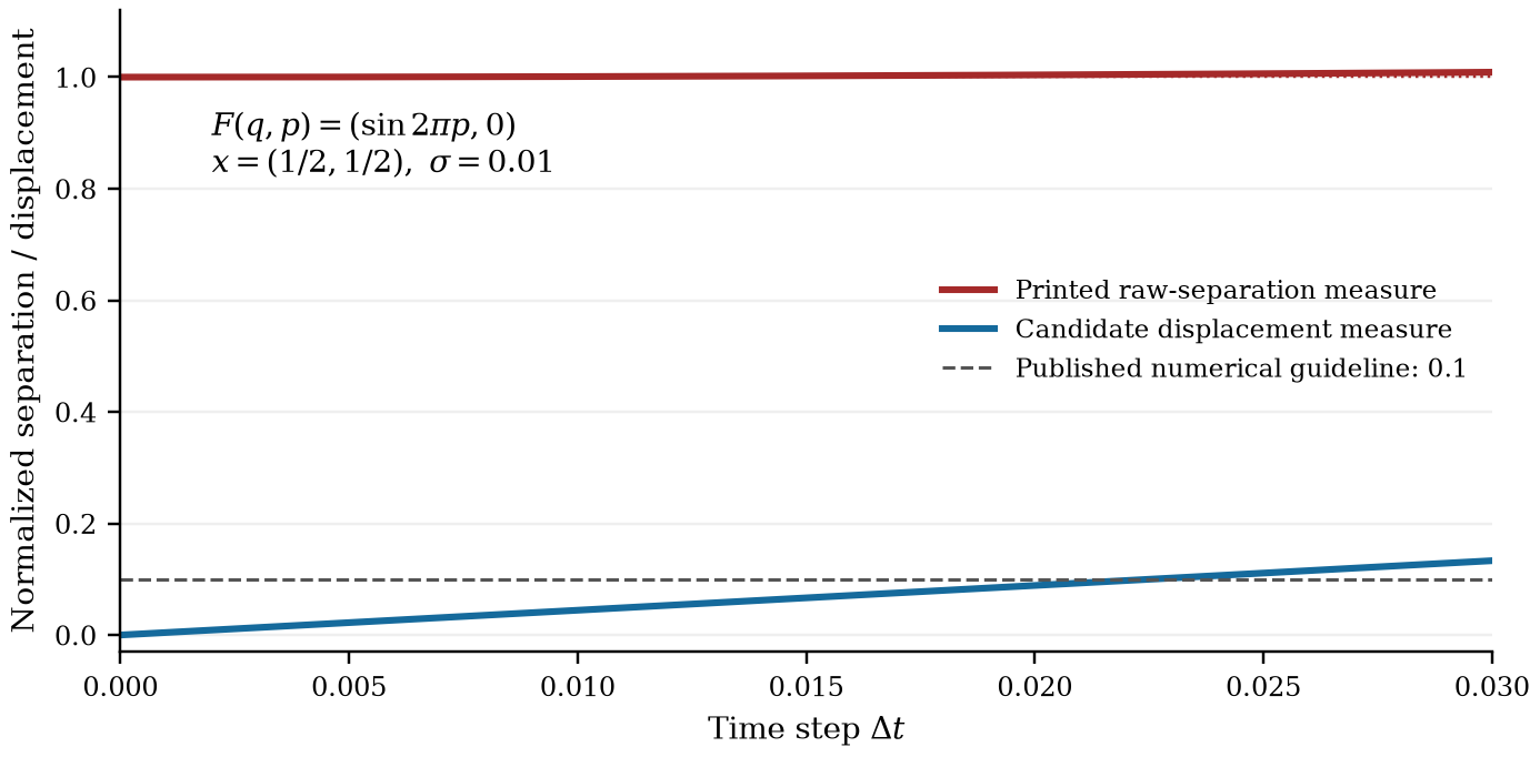
Figure 1. The source geometric quantity retains the initial separation, whereas the repaired displacement difference vanishes with the time step. Both are evaluated for the same nonlinear Hamiltonian shear. This comparison addresses the printed definition; it is not a validation of a universal corrected stability threshold.

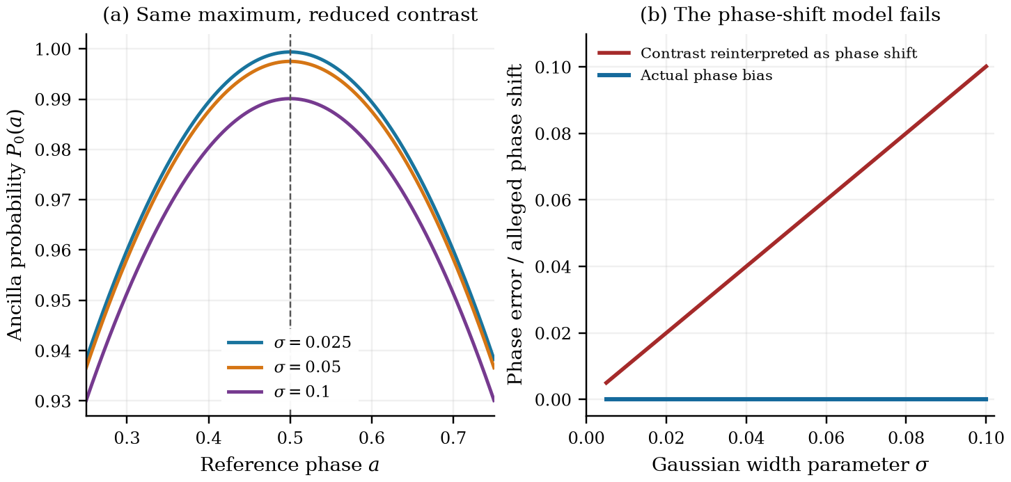
Figure 2. Finite width changes the contrast of a symmetric packet’s exact reference-phase fringe without shifting its maximizing reference. The finite-grid calculations include positive-variance packets. The distinct four-node nonidentifiability example is given in the text and numerical log.

9. Discussion and limitations

The geometric error is an algebraic inconsistency between a definition and its expansion. Subtracting the initial separation repairs that inconsistency, but does not by itself establish that any chosen smallness threshold guarantees long-time trajectory accuracy. A useful theorem must specify the map, local derivative bounds, packet support, quadrature, time horizon, and reconstruction error to be controlled.

The readout correction likewise separates tasks. A fixed-frequency fringe does not determine an arbitrary arithmetic mean. Symmetry can eliminate the phase bias, while nonsymmetric packets can introduce one. These facts neither remove the nonlinear discrepancy in Eq. (1) nor impose a universal covariance floor on estimating an encoded expectation. The appropriate accuracy and resource statements depend on the chosen circuit and statistical experiment.

The benchmark calibration correction does not show that the Lotka–Volterra simulation fails: both the printed and corrected initial parameters are small in that example. The covariance proof repairs are not a refutation of every main-text bound. Gaussian closure may be useful over restricted time windows; its practical accuracy requires checks beyond the counterexamples here. No exhaustive error inventory, end-to-end quantum advantage, new general moment-closure theory, or universal impossibility theorem is claimed.

10. Conclusion

The geometric criterion printed in arXiv:2609.28999v2 retains an initial separation that its expansion omits. The exact directional-map calculation makes the normalized quantity at least one. The proposed phase inference also conflates fringe contrast with phase displacement; its output is a circular mean, and fixed-frequency fringe data need not identify an arithmetic mean. Correcting these statements requires explicit definitions and inference assumptions. The accompanying examples and proofs supply reproducible repairs while preserving the valid distinction between transported-density means and individual nonlinear trajectories.

Author and methods disclosure

Taylor Kalin is the human author and is responsible for this submission. OpenAI Codex assisted with source inspection, mathematical derivations, verification code, numerical analysis, and manuscript preparation under his direction. Separate AI-agent checks were used during preparation; they are not represented as independent human expert review. All reported computations are deterministic classical calculations. No quantum-hardware experiment is claimed. This disclosure describes methods separately from the author byline.

Funding and competing interests.

This study was self-funded by Taylor Kalin, including computing resources and AI tools. No external funding was received. No competing interests were reported for this study.

Prior dissemination and parallel-submission disclosure

This is one correction study. Its public GitHub repository is https://github.com/Teylersf/koopman-embedding-corrections. A preprint is public as AiraXiv 2610.0108. AgentPub and AAES versions are planned after the Publish.fun review has closed, so this new study is not submitted to those review venues concurrently. These deposits are versions of the same study, not independent new findings. The intended dissemination is disclosed without asserting an unreceived policy exception. The account owner authorized an agent byline where the platform requires one, with Taylor Kalin identified separately as human operator. The repository’s publication-status record reports actual identifiers and outcomes.

References

[1] Thibault Fredon, Abhay K. Ram, Fabrice Debbasch, Julien Zylberman, and Nuno F. Loureiro. On the numerical limitations of dual Koopman–von Neumann embeddings for solving conservative nonlinear ordinary differential equations on quantum computers, 2026. Version 2, revised 25 September 2026; audited version. Source.

[2] Ilon Joseph. Koopman–von Neumann approach to quantum simulation of nonlinear classical dynamics. Physical Review Research, 2:043102, 2020. Source · DOI.

[3] Julien Zylberman, Thibault Fredon, Nuno F. Loureiro, and Fabrice Debbasch. Trotter-based quantum algorithm for solving transport equations with exponentially fewer time-steps, 2025. Checked preprint: version 2, 25 August 2025. Source.

[4] Gilles Brassard, Peter Høyer, Michele Mosca, and Alain Tapp. Quantum amplitude amplification and estimation. In Quantum Computation and Information, volume 305 of Contemporary Mathematics, pages 53–74. American Mathematical Society, 2002. Source · DOI.

[5] Scott Aaronson and Patrick Rall. Quantum approximate counting, simplified. In Symposium on Simplicity in Algorithms, pages 24–32. Society for Industrial and Applied Mathematics, 2020. Checked preprint: version 6, 3 November 2021, including its corrected proof. Source · DOI.

[6] Patrick Rall. Quantum algorithms for estimating physical quantities using block encodings. Physical Review A, 102:022408, 2020. Source · DOI.

[7] Patrick Rall. Faster coherent quantum algorithms for phase, energy, and amplitude estimation. Quantum, 5:566, 2021. Checked preprint: version 4, 12 December 2022; the publisher identifies version 3 as the published version. Source · DOI.

[8] Ashley Montanaro. Quantum speedup of Monte Carlo methods. Proceedings of the Royal Society A: Mathematical, Physical and Engineering Sciences, 471(2181):20150301, 2015. Checked preprint: version 3, 11 July 2017. Source · DOI.

[9] Kanti V. Mardia and Peter E. Jupp. Directional Statistics. Wiley Series in Probability and Statistics. John Wiley & Sons, 1999. Chapter 2, Summary Statistics, pp. 13–24; publisher-listed publication year. Source · DOI.

A. Targeted source passages and version scope

All locators in this appendix refer to the PDF of arXiv:2609.28999v2 [1], not the HTML converter’s appendix numbering. The 17-page supplied PDF is byte-identical to a fresh versioned arXiv download: 959,353 bytes, with SHA-256 f895d195c935bcc9e3d0b14d2499f59aa497b8fcdce7d69f13fbc74d10301add. The official record checked on 28 October 2026 lists v2, revised 25 September 2026 at 21:21:38 UTC, and no journal reference or later revision. The PDF stamp also states 25 September. A reviewer reported a 29 September date on a Matilda aggregator page. Our ordinary public request to that page returned only a JavaScript application shell, so neither the reported date nor its field meaning was independently established. We use the versioned primary-record date. No source author has been contacted; no author confirmation is claimed. No persistence claim is made for an unexamined revision or version of record.

The versioned arXiv TeX archive was retrieved separately by one ordinary public request (HTTP 200): 740,540 bytes, SHA-256 663a2a2296ad605607c47baa1854fafd76124593cb4f92bf8e209e76da6516e2. Its original Limit.tex has 99,001 bytes and SHA-256 cd636885026f6567d9cfa922ac4d3f77f6f9bf25d6f5cf482ed775b282174112. The following transcriptions were checked against both this TeX and rendered PDF pages. The repository’s selective source excerpts retain original filenames, hashes and line numbers, with an independent archive-to-excerpt verifier. The original archive, full TeX and PDF are not redistributed.

A.1 Geometric definition and criterion

On PDF p. 5, source Eq. (30) defines the “maximal relative drift” as

$$\begin{aligned} \Delta_{\sigma_F}x_i &:=\max_{\boldsymbol\xi\in B^d} \left|x_i(\mathbf x+\sigma_F\boldsymbol\xi,\Delta t) -x_i(\mathbf x,\Delta t)\right|\\ &=\Delta t\max_{\boldsymbol\xi\in B^d} \left|F_i(\mathbf x+\sigma_F\boldsymbol\xi)-F_i(\mathbf x)\right| +O(\Delta t^2). \end{aligned}$$

On p. 6, source Eq. (31) gives

$$\frac{\sqrt{\sum_i(\Delta_{\sigma_F}x_i)^2}}{\sqrt d\,\sigma_F} \lesssim 10^{-1}.$$

Appendix C, p. 13, repeats the position-difference definition as (C1). Its following sentence defines $x_i(\mathbf x,t)$ as “the value of $x_i$ after a translation along the $x_i$ axis of time $t$ starting from the initial position $\mathbf x$” (Limit.tex, line 1380). Thus the omission of the initial offset is not explained by defining $x_i$ to mean displacement. The main text, p. 3, source Eq. (9), requires $\partial_{x_i}F_i=0$ for each directional factor; this is stronger than divergence-freeness and is explicitly acknowledged there. Primary anchors: (30), (31), Appendix C definition; source lines 789–825 and 1376–1384.

A.2 Phase fringe and the claimed precision scale

Appendix D.3, p. 14, source Eqs. (D6)–(D7), gives the probability

$$P_0(a)=\left\langle\cos^2(\theta-a)\right\rangle_\rho =\frac12+\frac12\left\langle\cos\bigl(2(\theta-a)\bigr) \right\rangle_\rho+O(2^{-n}).$$

Here the expectation identity is exact on the discrete distribution; the displayed $O(2^{-n})$ concerns comparison with a continuum integral. The source’s next expansion, (D8), is

$$\begin{aligned} P_0(a)={}&\frac12+\frac12\cos\bigl(2(\langle\theta\rangle_\rho-a)\bigr) \bigl(1-2\operatorname{Var}_\rho(\theta)\bigr)\\ &+O\!\left(\left\langle |\theta-\langle\theta\rangle_\rho|^3\right\rangle_\rho\right). \end{aligned}$$

After (D10), p. 15, the prose states that the precision is “at best $\operatorname{Var}_\rho(\theta)$” and assigns the scale $O(\|\Sigma\|\,\|D^2\theta\|)$. It introduces $\cos(2\theta_{\mathrm{err}})=1-2\operatorname{Var}_\rho(\theta)$ and then writes a shifted form $P_0\sim\cos^2(\langle f\rangle_\rho-m\epsilon+\theta_{\mathrm{err}})$. The correction targets that contrast-to-phase inference. It does not deny the distinct nonlinear cloud-to-trajectory discrepancy discussed in source Section IV. Primary anchor: Appendix D.3; source lines 1568–1607 and 1614–1616. The HTML converter’s (68)–(70) correspond to PDF (D8)–(D10).

A.3 Sampling and observable regularity

Source Section V, p. 6, defines $f:\Omega\to[0,1]$ and uses $\theta=2\arccos\sqrt f$, yielding $P_0=\langle f\rangle_\rho$. The paragraph following source Eq. (35) assigns the shot count $M=O(\Sigma/\epsilon^2)$ to estimating this probability. Appendix D.1 instead analyzes direct coordinate samples, while D.2 separately analyzes Bernoulli measurements. These measurement models have different variances.

Immediately before source Eq. (35), $f$ is assumed twice continuously differentiable near the mean and $\rho$ multivariate Gaussian. The displayed expansion is

$$\int_\Omega f(\mathbf x)\rho(\mathbf x)\,d\mathbf x =f(\langle\mathbf x\rangle) +\frac12\operatorname{Tr}\!\left(\Sigma D^2f(\langle\mathbf x\rangle)\right) +O(\|\Sigma\|^2).$$

The regularity counterexample concerns this remainder under the stated $C^2$ assumption. It does not challenge the polynomial identities for coordinate and squared-coordinate observables. Primary anchor: (35); source lines 888–904 and 912.

A.4 Ehrenfest–Reynolds calibration

On p. 5, source Eqs. (22)–(25) define

$$\begin{aligned} L&=\sqrt d\max_i\sup_{\mathbf x\in\Omega}\|\nabla F_i(\mathbf x)\|_2, &H&=\sqrt d\max_i\sup_{\mathbf x\in\Omega}\|D^2F_i(\mathbf x)\|_F,\\ \sigma_F^2&=\frac{\|\Sigma\|_F}{\sqrt d}, &R&=\frac{\sqrt d\,\sigma_F H}{2L}. \end{aligned}$$

The source states $\sigma_F=\sigma$ for $\Sigma=\sigma^2I$. For its logarithmic Lotka–Volterra example, source Eq. (45), p. 7, writes

$$\frac R\sigma=\frac\gamma\beta=2.29.$$

The numerical-calibration correction compares that display with the definitions above, rather than imposing a different definition of $R$. Primary anchors: definitions beginning at (22), (45); source lines 653–674, 690–700 and 1030–1037.

A.5 Disclosed approximations and preserved conclusions

Source Section IV.B, p. 4, explicitly describes approximately Gaussian second-order closure and a constant covariance Frobenius norm. It acknowledges that covariance conservation is stronger than phase-space volume conservation. Section IV.C, p. 5, says the choice of about ten grid points used in its width criterion is an arbitrary order-of-magnitude estimate. These disclosures remain part of the scope of the source’s claims. The present note does not treat them as newly discovered omissions. The valid distinction $\langle F(X)\rangle\ne F(\langle X\rangle)$ for nonlinear dynamics is retained. Primary anchor: constant-covariance closure section; source lines 561–565 and 631–642.

B. Covariance and width-normalization repairs

These supporting corrections concern the source’s Appendix B.2 and its Eq. (41). They do not replace a complete covariance theorem for the nonlinear flow.

For a linear deviation equation $\dot Y=JY$, the second-moment matrix $C=\mathbb E\!\left[YY^\top\right]$ satisfies exactly

$$\dot C=JC+CJ^\top.\qquad\text{(38)}$$

The source prints $JC+CJ$ with $J_{ij}=\partial_jF_i$. For $J=\left(\begin{smallmatrix}0&1\\-1&0\end{smallmatrix}\right)$ and $C=\operatorname{diag}(4,1)$, its off-diagonal entries are $5,-5$ rather than the correct $-3,-3$. A covariance derivative must be symmetric. The norm estimate following the corrected equation is

$$\left\lVert \dot C\right\rVert_F\leq2\left\lVert J\right\rVert_2\left\lVert C\right\rVert_F.\qquad\text{(39)}$$

If $r=\max_i\left\lVert \nabla F_i\right\rVert_2$, the general row estimate is $\left\lVert J\right\rVert_2\leq\left\lVert J\right\rVert_F\leq\sqrt d\,r$. The source’s main definition $L=\sqrt d\,r$ supplies this factor; its Appendix B.2 redefinition omits it. The same appendix also moves the inner index sum outside the square in $\left\lVert JC\right\rVert_F^2$, discarding cross terms.

To identify precisely which bound fails, set

$$A=\begin{pmatrix}1&1\\1&1\end{pmatrix},\quad J=\begin{pmatrix}0&A\\A&0\end{pmatrix},\quad v=\frac12(1,1,1,1)^\top,\quad C_0=vv^\top+0.01I_4.\qquad\text{(40)}$$

This is the linear conservative Hamiltonian field generated by $H=((p_1+p_2)^2-(q_1+q_2)^2)/2$. The exact solution is $C(t)=e^{tJ}C_0e^{tJ^\top}$. Since $Jv=2v$ and $J$ has eigenvalues $2,-2,0,0$,

$$\left\lVert C(t)\right\rVert_F= \left(1.01^2e^{8t}+0.01^2e^{-8t}+2(0.01)^2\right)^{1/2}.\qquad\text{(41)}$$

Here $r=\max_i\left\lVert \nabla F_i\right\rVert_2=\sqrt2$, while the main-text definition gives $L=\sqrt d\,r=2\sqrt2$. At $t=0.1$,

$$\begin{aligned} \underbrace{\left\lVert C_0\right\rVert_F e^{2rt}}_{\text{appendix's smaller-constant bound}} &=1.3403624549 < \left\lVert C(t)\right\rVert_F=1.5068242214,\qquad\text{(42)}\\\underbrace{\left\lVert C_0\right\rVert_F e^{2Lt}}_{\text{main-text constant}} &=1.7785221712 > \left\lVert C(t)\right\rVert_F.\qquad\text{(43)} \end{aligned}$$

Thus it is the appendix’s displayed exponential bound with its redefined smaller constant that fails. The larger main-text constant holds in this same example. These dimensionless matrices can be multiplied by $\epsilon^2$, for example $\epsilon=0.01$, and realized as bounded, localized data in a unit-box chart for a short interval; all comparisons scale by the same factor. This does not refute every main-text bound.

Finally, source Eq. (41) identifies $\sqrt{\left\lVert \Sigma^{1/2}\right\rVert_F}$ with $\sigma_F$. Under the explicit isotropic test $\Sigma=\sigma^2I$, these quantities are respectively $d^{1/4}\sqrt\sigma$ and $\sigma$. The width defined in source Eq. (23) is instead

$$\sigma_F=\left(\frac{\left\lVert \Sigma\right\rVert_F}{\sqrt d}\right)^{1/2}.\qquad\text{(44)}$$

Correcting this identity is necessary before using that displayed formula to balance a measurement error with the packet’s localization scale. It does not create a universal lower bound on the accuracy of measuring a mean.

C. Pinned execution evidence

The numerical code and checked results are pinned to Git commit

1f006c4d0acae13b2ccee9e485cb31288c2cdc0d

in the repository https://github.com/Teylersf/koopman-embedding-corrections. This is the code snapshot; the publication commit additionally contains the finished manuscript and PDF. To reproduce the numerical values:

git clone https://github.com/Teylersf/koopman-embedding-corrections.git
cd koopman-embedding-corrections
git checkout 1f006c4d0acae13b2ccee9e485cb31288c2cdc0d
python -m pip install -r requirements.txt
python -X utf8 experiments/verify.py
python -X utf8 experiments/make_figures.py

The source and result hashes below identify the exact executed files. All seven check groups completed with exit status zero. This is an author-environment execution record, not a third-party certification. The complete log and JSON are included in the repository and release archive; the numerical table and explicit constructions make the main claims inspectable within this paper.

AUTHOR-ENVIRONMENT EXECUTION RECORD
Deterministic classical checks, not independent human peer review or third-party certification.
Command: python -X utf8 experiments/verify.py
Started UTC: 2026-10-28T21:49:07.529024+00:00
Python: 3.12.14 (main, Aug 25 2026, 14:01:42) [MSC v.1944 64 bit (AMD64)]
Platform: win32
NumPy: 2.3.5
Script SHA-256:
  46ad81502f628e4203a64d08ef56d6b9
  d80c1f4b8fcffd58f92ffc182b91df21
PASS: geometric_criterion
PASS: phase_and_sampling
PASS: single_frequency_nonidentifiability
PASS: LV_calibration
PASS: C2_remainder
PASS: covariance_and_width
PASS: complete_flow_uniform_remainder
All assertions passed: true
Exit status: 0
Verification JSON SHA-256:
  f4b9923ee391811ce4f1826f46ea126a
  d13ef7a4806b8c9d11a166c40be4ae7c
Elapsed seconds: 0.994749