Abstract
This diagnostic comment examines initial-state matching and pressure realizability in arXiv:2607.07106v1. Its exact mixture identities are correct. However, archived PIC and fluid initial moment-current profiles differ by $9.87\%$ in the full-domain, $x$-averaged relative $\ell^2$ norm; local Cartesian covariance pressures differ by about $20\%$ in $P_{xx}$ and $38.4\%$ in $P_{zz}$. The PIC input specifies proper momentum where the fluid input specifies ordinary velocity. Complete archive checks and independent ten-moment layout validation corroborate the data audit. Four clean-source fluid cases attempt comparisons of the posted and aggregate-PIC-matched initializations, while distinguishing the unavailable historical dirty build. At identical one-fluid endpoint times, matching lowers $P_{xx}$ error against PIC from $36.29\%$ to $28.85\%$, with smaller errors in density, current and $P_{zz}$ as well. These are numerical endpoint results, not validated physical dynamics: both one-fluid cases contain indefinite covariance tensors at saved intermediate times, and the clean unmatched two-fluid endpoint is also inadmissible. The matched two-fluid run terminates with an invariant-check assertion before producing its comparison endpoint. The clean implementation tests coordinate pressures without testing full tensor positivity. The original archived endpoints pass the same covariance checks; their intermediate trajectories and exact executable remain unidentified. A conditional loader calculation, an auxiliary homogeneous stability benchmark, a continuity clarification and a cancellation-conditioned heat-flux bound provide separate diagnostics. The results motivate matched moments and realizability checks without disproving the source’s exact algebra or establishing that its nonlinear physical conclusions are false.
Editorial notes
Points the editor recorded on accepting the paper. They are published with the article; the authors were not required to address them before publication.
- Figure 6: replace the stored link to up_OpSH28VIOyPCC4-z/figures/figure-2.png with a uniquely named stability-spectrum file, and state in the caption or Section 8 that its content was verified.
- Section 3.4 and Abstract: discuss explicitly that the matched one-fluid case has more saved non-PSD instances (5/31 vs 3/31 in Table 2) and a more negative minimum eigenvalue, so that readers weigh the endpoint gains against faster realizability loss.
- Section 3.1: report whatever is recoverable about the MomentSpecies.lua:495 assertion in the matched two-fluid run (the invariant checked and the last valid frame's minimum population eigenvalue) to support diagnosis by others.
- Section 8 and reference [2]: keep the DataCite registration note and direct record links, since the Crossref-only reference check still reports both Zenodo DOIs as not_found.
- Sections 5 and 6: condense the continuity clarification, which the paper itself labels standard kinematics, so that Sections 2–3 carry the paper's emphasis.
Initial-state matching and pressure realizability in counter-streaming electron-fluid comparisons
Taylor Kalin
taylorkalin.com · teylersf@gmail.com · ORCID: 0009-0003-9000-9315
28 October 2026 · Version 1.2.0
Abstract
This diagnostic comment examines initial-state matching and pressure realizability in arXiv:2607.07106v1. Its exact mixture identities are correct. However, archived PIC and fluid initial moment-current profiles differ by in the full-domain, -averaged relative norm; local Cartesian covariance pressures differ by about in and in . The PIC input specifies proper momentum where the fluid input specifies ordinary velocity. Complete archive checks and independent ten-moment layout validation corroborate the data audit. Four clean-source fluid cases attempt comparisons of the posted and aggregate-PIC-matched initializations, while distinguishing the unavailable historical dirty build. At identical one-fluid endpoint times, matching lowers error against PIC from to , with smaller errors in density, current and as well. These are numerical endpoint results, not validated physical dynamics: both one-fluid cases contain indefinite covariance tensors at saved intermediate times, and the clean unmatched two-fluid endpoint is also inadmissible. The matched two-fluid run terminates with an invariant-check assertion before producing its comparison endpoint. The clean implementation tests coordinate pressures without testing full tensor positivity. The original archived endpoints pass the same covariance checks; their intermediate trajectories and exact executable remain unidentified. A conditional loader calculation, an auxiliary homogeneous stability benchmark, a continuity clarification and a cancellation-conditioned heat-flux bound provide separate diagnostics. The results motivate matched moments and realizability checks without disproving the source’s exact algebra or establishing that its nonlinear physical conclusions are false.
1 Introduction and scope
Counter-streaming electron populations provide a useful representation of the strongly non-Maxwellian distributions generated during collisionless magnetic reconnection. McGrae-Menge and collaborators [1] report that tagging electrons by their initial side of a current sheet isolates sub-populations whose intrinsic third moments are small compared with their combined heat flux. Their exact moment decomposition explains how relative motion and population asymmetry can generate a substantial aggregate third moment even when each population has little intrinsic heat flux. Evolving additional population moments is therefore physically motivated.
The principal contributions are an initial-state audit and clean-source numerical tests with explicit covariance-realizability checks. Equal nominal drift and temperature parameters need not specify equal laboratory-frame moments in a relativistic particle initializer and a nonrelativistic fluid initializer. The new evolutions quantify numerical endpoint sensitivity, while their saved-state failures limit physical interpretation and do not identify the source’s unavailable historical executable.
Our first result uses the authors’ publicly archived initial moments and input decks [2]. Identical nominal drift expressions enter a proper-momentum initializer in PIC and an ordinary-velocity initializer in the fluid model. The recorded initial moments show a current and pressure mismatch consistent with that distinction. This is a reproducible control issue for interpreting the nonlinear comparison; its eventual dynamical effect cannot be determined from initial-state analysis alone.
Four prescribed clean-source cases extend that audit. Matching aggregate PIC moments reduces one-fluid endpoint errors, but both one-fluid histories contain non-realizable saved covariance tensors. The clean unmatched two-fluid endpoint also fails the full covariance check. Its primary error metrics are withheld. The implementation’s diagonal-only acceptance test does not detect these failures. We therefore distinguish numerical endpoint contrasts from validation of a physically admissible trajectory.
An auxiliary result is a controlled longitudinal stability test of the stated continuum isotropization closure. A positive two-Maxwellian equilibrium is stable to longitudinal electrostatic perturbations under the established Penrose criterion [3], but its finite-relaxation fluid counterpart has an overstable mode. We give an explicit linear system and check both its eigenvalue residual and Gauss constraint. The test is homogeneous and nonrelativistic. It does not replace the source’s inhomogeneous reconnection calculation, refute its application-specific instability-capability statement, or show that the identified mode caused any of its plotted features. The source populations initially share a velocity; the counter-streaming equilibrium used in this calibration test is different.
Two secondary observations make the interpretation more precise. Continuity depends on the divergence of the mass flux, so a zero normal velocity at a symmetry plane does not prohibit density accumulation there. A conditioned third-moment error bound also shows why a thermal-to-drift speed ratio alone does not give a universal relative-error guarantee when population contributions cancel. Neither result disputes the empirical parameter trend in the published scan.
1.1 Relation to established work
Heat-flux closure and its effect on collisionless response are established subjects. Hammett and Perkins [4] developed fluid moment models for Landau damping, while Wang and collaborators [5] compared multifluid moment models with PIC reconnection. Goldman and collaborators [6] studied multibeam energy moments and the distinction between component and aggregate centering. The mixture algebra used below belongs to this established moment framework.
Closure-dependent instability spectra are also known. Ng and collaborators [7] demonstrate why a pressure-tensor model must be checked against kinetic response rather than judged solely by its retained variables. Our finite-relaxation example supplies a concrete test associated with the closure and reference rate in the present source; we do not claim the general phenomenon of closure-dependent unstable modes as new.
Work on heat-flux closure for nonlinear electrostatic two-stream systems [8, 9] further limits a literal reading of broad claims that no fluid closure can capture non-Maxwellian counter-streaming. It does not establish prior use of the specific tagged-population closure in electron-only reconnection. Our analysis therefore addresses explicit initialization, realizability, continuity and stability statements, and preserves the source’s application-specific empirical evidence.
1.2 Audited version and available evidence
The supplied ten-page PDF is byte-identical to a fresh versioned download of arXiv:2607.07106v1: 7,847,791 bytes, SHA-256 fc5344e2ba8f4db98baf90d805bb6b7ce8835c32ea7bf54bba4d62f405b955a3. The official history checked on 28 October 2026 lists the 8 July v1 and no later revision or journal reference. The PDF displays 9 July, while the experimental HTML displays a different compilation date. The original TeX uses \date{\today}; those compilation dates do not identify additional scientific revisions. Appendix A records source and data locators. No original author has been contacted, and no author confirmation or private simulation-build access is claimed.
2 Initial-state matching in the supplied input decks
The source compares a relativistic PIC calculation with nonrelativistic ten-moment fluid calculations and describes their common initialization in Appendices A and C [1]. The deposited reference-case decks and initial moments make the physical matching of those states directly testable [2]. Equal numerical drift and temperature parameters need not specify equal laboratory-frame velocity moments in the two codes. This issue concerns the controlled comparison; the mixture identities do not depend on either code’s initialization convention.
2.1 A proper-momentum parameter is used as a fluid velocity
The PIC deck sets use_spatial_ufl=.true. and supplies the curl-derived drift expressions as spatial_ufl. The official OSIRIS reference defines these inputs as proper velocities, or momentum divided by particle mass, with relativistic boosting as the default [10]. No classical-addition override appears in the posted deck. The Lua decks instead set nonrelativistic conserved momentum density to using the same expressions. This is the ordinary velocity variable of the ten-moment equations [5].
Writing , a cold population with proper drift has
Thus the same numerical vector used for in PIC and in the fluid initializer does not match the physical cold drift. At the unperturbed lower sheet center, the reference expressions give approximately : the cold PIC speed is , whereas the prescribed fluid speed is . The fractional difference is . It persists when the thermal spread tends to zero at fixed and sheet width ; low thermal beta alone does not remove it. Equation (1) is a cold-limit explanation. A finite-temperature mean must be measured after loading rather than identified with that limit.
2.2 A conditional finite-temperature loading calculation
The complete 155-line posted PIC deck contains two thermal-distribution blocks with , and no classical-addition override or include directive. The inspected public OSIRIS loader draws independent Gaussian thermal proper-momentum components and boosts each particle without changing its weight [11]. With , for thermal momentum and proper drift , this rule is
This is a prediction conditional on the public loading rule, not an identification of the original executable. With and , pairing opposite Gaussian momenta gives
for positive drift and nonzero thermal spread. Thus the mean can fall below the cold conversion without an additional force. An invariant scalar distribution sampled at equal laboratory time would require a different Jacobian-weighted measure; it must not be silently substituted for this unweighted sample-boost rule.
At the finite-temperature mean is , below the cold . Evaluating the full spatial drift expressions and perturbations at the two lower diagnostic rows gives an -averaged zero-shape prediction . A separate, unfitted sensitivity uses the declared quadratic interpolation, the recorded moment-cell offset and the posted regular particle lattice. Summing the standard quadratic weights over their support gives the following conditional values:
| Quantity | ||
|---|---|---|
| Archived | 0.44098722 | 0.44087669 |
| Pointwise loading prediction | 0.44197416 | 0.44197416 |
| Quadratic-shape prediction | 0.44098868 | 0.44098868 |
| Archived | 0.00994868 | 0.00997543 |
| Quadratic-shape | 0.00996490 | 0.00996490 |
| Archived | 0.00769653 | 0.00769303 |
| Quadratic-shape | 0.00770632 | 0.00770632 |
These pressure predictions use expected raw moments centered at each node before averaging, in the infinite-particle limit. No temperature, drift, shape width or perturbation is fitted to the archived values. Quadrature orders 12, 20, 32 and 48 agree in the quadratic mean to about ; an independent Cartesian quadrature checks the reduced moment calculation to in the tested quantities. This is a conditional consistency check of the scale of the additional reduction below the cold value. Agreement does not identify the historical loader or the custom diagnostic kernel. The standard public deposition kernel is not verified as the original custom velocity diagnostic’s kernel, so the pointwise prediction and shape sensitivity remain distinct. Neither is a new PIC run or a confidence statement about the unidentified original build.
2.3 Archived initial current and staggered magnetic curl
The original data authors explicitly define the archived diagnostic vfl_i as [2]. It is therefore an ordinary mean velocity, even though the input parameter ufl is a proper-momentum parameter. With the source normalization , the physical moment current is
The selected initial density diagnostics give to within . No particle tracking or new time integration is needed to evaluate this current.
The HDF5 files also record their grid offsets: density and velocity moments have , has and has . The backward staggered differences therefore place
on the moment-cell centers. Periodic differencing makes the first term’s average exactly zero. The raw data use ; the paper’s coordinate is , so its lower sheet is at .
Table 1. Initial -averaged currents in the cells adjoining the lower sheet. The deficit is . Currents use the source’s normalized units.
| Deficit | |||
|---|---|---|---|
| 15.95 | |||
| 16.05 |
The supplied fluid initializer prescribes an -averaged ordinary velocity in these same cells. The archived PIC means are and , approximately smaller. The small difference between this continuum prescription and Table 1’s staggered curl does not explain the observed deficit. The adjacent cells at the other sheet show the same effect with reversed current sign.
The result is not restricted to these four illustrative cells. Across all 640 rows, the relative discrepancy between the -averaged moment-current and Yee-curl profiles is . Restricting to or gives and , respectively. These are norms of the one-dimensional averaged profiles, not norms of the full two-dimensional fields. Figure 2 displays both sheets and the full domain. The input-prescribed current differs from the Yee profile by only in the full-profile relative norm.
As a deterministic discretization sensitivity, averaging the staggered fields onto cell centers before a centered derivative changes the curl profile by in that norm. This is a deliberately smoothed representation, not an alternative reading of the recorded Yee offsets. The central-cell moment-current deficits remain about – against that smoothed profile. Eight contiguous 60-column blocks at have moment-current means between and , compared with the Yee mean . The per-column standard deviation is . These spatial summaries are descriptive; correlated particle deposition and the imposed perturbation preclude treating them as independent-sample confidence intervals.
Here is a moment-based physical diagnostic. We have not reloaded OSIRIS’s native charge-conserving deposited current, which can differ from a simple deposition. These numbers therefore do not specify the exact discrete electric-field update of the original executable. In the normalized continuum equations, . The comparison is a continuum magnetostatic diagnostic. It does not establish an initial transient in the native numerical electric-field update.
2.4 The laboratory-frame pressure moments also differ
The record defines its second-moment diagnostics without a density normalization: [2]. Following the source’s own pressure definition, at we compute
The posted fluid initializers prescribe an isotropic thermal pressure
The archived initial fluid .bp fields independently confirm this pressure in both fluid models, as detailed below. The measured ratios to the archived fluid pressure are
| 15.95 | 0.795900 | 0.615727 |
| 16.05 | 0.798040 | 0.615447 |
For example, at the archived values are and . The latter is about below the archived fluid pressure. These are the ordinary-velocity covariance moments defined in the source, not components of a relativistic energy–momentum tensor. A common rest-frame thermal-momentum parameter does not imply equal laboratory-frame velocity covariance after a boost. Centering the pressure after averaging in instead adds the density-weighted variance of the resolved mean flow. At the four central rows this changes either diagonal component by approximately , far smaller than the reported pressure mismatch; the source definition and our principal result center each cell first. Figure 1 shows the local -averaged profiles.
2.5 Corroboration against the saved fluid state
We reloaded five initial BP snapshots: the one-fluid electron state, both two-fluid electron states, and each model’s electromagnetic field. They record time and frame zero, a single available step, the same grid and bounds, zero ghost cells and polynomial order zero. Each file’s embedded base64 input deck decodes byte-for-byte to the posted Lua file. This checks the input used in the saved output, rather than assuming that the separate prescription was executed unchanged.
The ten stored components are , the three , and the six symmetric raw second moments. Their order independently matches the official Gkeyll conservative-variable layout [12] and is checked against every returned initializer component over all 307,200 cells, including off-diagonal moments and the field components. The largest one-fluid component error is ; the summed two-fluid state differs from the one-fluid state by at most . Aggregate pressure is reconstructed after summing the conservative population moments. Thus the earlier comparison with the prescribed initial state is corroborated by the actual archived state.
Against either reloaded fluid model, the full 640-row, -averaged PIC profiles have relative differences of for , for and for . At the two lower central rows the actual fluid current is , giving moment-current deficits and . The local pressure ratios reported above are unchanged. These comparisons concern physical velocity moments, not native PIC current deposition or later-time dynamics.
All selected PIC files have TIME=0 and ITER=0; the fluid files have time and frame zero. No explicit time-averaging attribute appears. This verifies the posted snapshot metadata, not the impossibility of an undocumented operation in the unidentified PIC build. A complete inventory of all 223 PIC ZIP entries, including 94 scientific files, identifies no native deposited-current diagnostic. We therefore cannot make the requested native-current comparison from this deposit and do not substitute the UDIST moment current for it.
2.6 What a controlled comparison requires
The data establish an initial-state mismatch in the posted comparison. They do not establish how much of any later reconnection difference it causes. That requires reruns with controlled initial moments and numerical refinement. One constructive test is to initialize the fluid models from the measured PIC , and , preserving the intended population labels. Another is to calibrate the PIC loading to a prescribed physical fluid state and then verify the deposited moments. The cold conversion in Eq. (1) is necessary for a cold drift match, but by itself does not guarantee a finite-temperature pressure or current match.
The fluid BP metadata records Gkeyll changeset 9663ea594e80+; its plus suffix does not identify a clean exact source tree or executable. The original PIC executable remains unidentified. The current public OSIRIS code inspected for documentation does not expose the authors’ custom vfl/third-moment diagnostic implementation. Our diagnostic interpretation follows their explicit dataset definitions and file metadata. The selected files in this section are initial snapshots. Their archived-data reanalysis is distinct from the new clean-source fluid evolutions in Section 3; it supplies no causal attribution of the source’s later nonlinear results by itself.
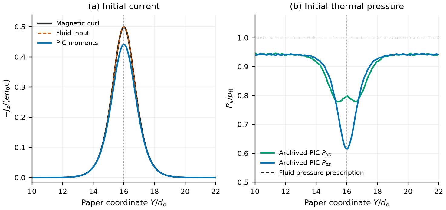
Figure 1. Reanalysis of the archived initial state near the lower sheet. Left: the ordinary-velocity moment current differs from both the staggered magnetic curl and the posted fluid prescription. Right: the local centered pressure components, averaged in after centering, differ from the isotropic fluid pressure. The profiles use the authors’ archived diagnostics and their published definitions [2]. The drawn fluid curves use the initializer; the reloaded initial fluid output independently corroborates them to roundoff. No new simulation is shown.
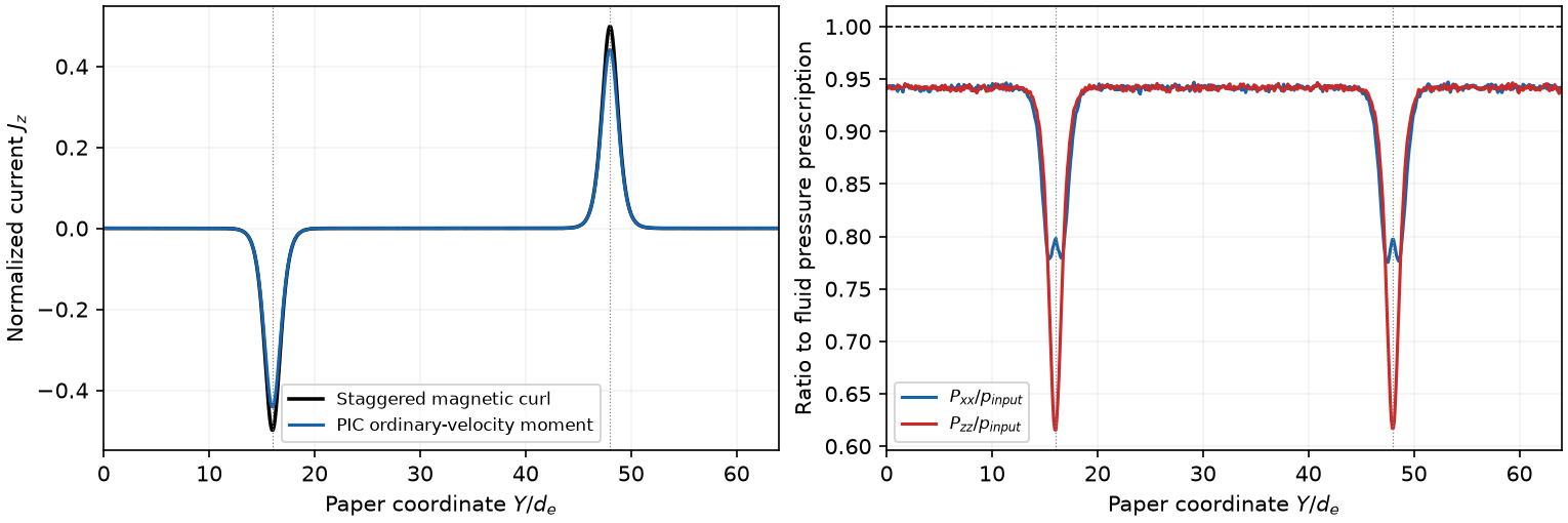
Figure 2. Full-domain, -averaged archived PIC profiles at , with both current sheets visible. Left: physical moment current and the correctly staggered magnetic curl. Right: velocity-covariance pressures divided by the fluid pressure confirmed in the archived output. The figure extends the local view; it is neither an independent simulation nor a native deposited-current diagnostic.
3 Matched-initial-state fluid comparisons
3.1 Intervention and implementation
The initial-state discrepancy motivates an initialization sensitivity experiment with both fluid models. The four cases use the posted one- and two-fluid initializers and aggregate-PIC-matched versions of each. The four-case intervention, solver settings and primary endpoint measurements were pinned before evolution. The matched state contains the archived PIC density, three ordinary-velocity momentum densities and six uncentered second moments at every cell. No smoothing, pressure repair or fitted drift correction is applied. The original electromagnetic fields, domain, grid, periodic boundaries, time stepper, CFL, closures and source terms are retained.
For two fluids the original smooth positive weights multiply the entire aggregate conserved vector. With and , this preserves the aggregate state and gives common velocity and population pressures . It matches aggregate moments through second order, rather than the PIC’s sharp tags, full distributions or intrinsic third moments. The intervention also imports sampled spatial variation. Its later effect cannot be attributed to the current mismatch, proper-momentum convention or thermal spread alone.
The tested Gkeyll implementation is built from clean source commit 9663ea594e80. All 1,998 native and Lua source files are unchanged; the source archive, compiler/dependency locks, installed runtime and executable hashes are recorded. The archived identifier 9663ea594e80+ does not identify its local changes or a unique executable. The clean baseline is therefore compared with the saved source-fluid state before interpreting the matched comparison. A compatibility failure with an older 2020 binary was retained; that binary supplies none of the new evolution results.
Native initial-output tests reproduce the original arrays bit-for-bit. The matched one-fluid conserved vector agrees bit-for-bit with its target. Both matched two-fluid splits agree bit-for-bit with their weighted targets; their aggregate differs by at most , with pressure error at most . All eight stored field components are unchanged. Every tested initial fluid population and aggregate PIC target passes positive-density and positive-definite covariance-pressure checks. These conformance tests do not establish identity with the historical dirty build.
Each case preserves tEnd=600, nFrame=60 and the original MPI decomposition. Gkeyll’s output trigger acts after accepted steps, without forcing an exact output time. A native stop request is issued only after the regular frame-30 files are closed, stable and consistent in their stored metadata; their hashes are checked again after process exit. Subsequent frames are excluded. Native rank logs and console output are also checked for the fatal timestep-collapse marker, including when a numerical failure returns exit code zero. An absent or failed case cannot supply a paired measurement. Three cases reach guarded regular frame 30. The matched two-fluid run instead exits with code 1 after an assertion in MomentSpecies.lua:495, without a native stop request or regular frame 30. Its last closed regular output is frame 22 at . That is a saved-output time, not the exact assertion time. The logged transient does not establish the failing cell, population or numerical cause. No final comparison or full saved-history pressure audit is inferred for this failed run.
3.2 Comparison quantities and scope
Unit electron mass and charge give . We recover aggregate pressure after summing the conserved population vectors. Current, density, and errors use every one of the 307,200 cells. Relative error is ; a zero reference norm gives an explicit null value, rather than an added small denominator. Separately reported profile norms first average over and can cancel transverse structure. They are not full-grid error norms. This is physical moment current, rather than the unavailable native deposited PIC current.
For two populations the reconstructable population-recentering contribution is
Its primary PIC comparator uses the deposited tag populations and documented first and second moments. This contribution depends on the decomposition. The finite local-isotropization model supplies a divergence, so it does not uniquely specify the complete intrinsic population heat-flux tensors. In particular, a one-fluid recentering contribution is zero by definition and does not imply zero full heat transport.
A separate central PIC reconstruction is conditional on treating the posted third-product diagnostics as unnormalized raw moments. The deposit explicitly defines its first/second diagnostics, but the third-product names and units do not verify that normalization. Algebraic reconstruction checks and this assumption are recorded separately. The four ordinary-moment comparisons and tagged- comparison do not depend on it. Exact-vacuum PIC tags contribute zero without a density floor. Their small negative diagnostic covariance eigenvalues, down to approximately and , are retained explicitly; the tag contribution is an algebraic diagnostic rather than certification of strictly positive-definite population states.
The PIC reference has stored time and iteration 4500. Source-fluid frame-30 times are and . New output times are likewise read from the files. Raw-frame comparisons use these actual times without interpolation. A matched frame number is not an exactly common physical time.
3.3 Realizability is stronger than positive coordinate pressures
For any nonnegative population distribution and any real vector ,
Consequently, covariance pressure must be positive semidefinite. Positive coordinate diagonals test only three directions; they do not impose this condition for every direction. The thermal-fluid comparison guard additionally requires strict positive definiteness.
The clean source’s TenMoment:isPositive in lines 128–136 checks density and the three recovered diagonal pressures for NaNs and negative values. It does not inspect off-diagonal components, principal minors or eigenvalues. MomentSpecies:checkInv applies that predicate cellwise and combines it across MPI ranks. The code’s primitive conversion independently confirms the off-diagonal packing, without an engineering factor of two.
The clean unmatched two-fluid endpoint gives a concrete witness. Population 1 has 16 indefinite cells, with . At the raw cell center its rounded covariance is
Density and all three diagonals are positive, but the unrounded dimensionless tensor’s principal minor is approximately and its determinant is . Independent long-double centering and quadratic form/minor checks corroborate the eigenvalue result. Population 2 and the aggregate remain positive definite. Aggregate positivity does not make an unrealizable component distribution admissible, so primary error metrics for this endpoint are withheld rather than computed after clipping or masking.
The corresponding original archived endpoint is positive definite in every cell of both populations and their aggregate. Its time is later by . The witness therefore establishes a failure of the identified clean reconstruction, not of the unavailable dirty build. The diagonal predicate makes normal native completion consistent with the failure; it does not identify the first loss time or the split operator that produced it.
Checking only initial and final states is also insufficient. The full saved-history audit was added after the clean two-fluid endpoint failed the strict collector; it is an additional diagnostic, not a prespecified primary performance measurement. A hash-bound scan of all regular saved frames 0–30 finds that the unmatched one-fluid case has 9, 18 and 7 indefinite cells at saved times near 220, 230 and 240, despite positive-definite endpoints. The matched one-fluid case has 5, 23, 47, 30 and 5 at saved times near 220–260. Their most negative eigenvalues are and in units of , respectively. The two-fluid unmatched population 1 also fails at saved frames 19 and 22, with two cells each, in addition to its rejected endpoint; its population 2 and aggregate pass all 31 saved checks. These are observed saved snapshots, not every accepted timestep or proof of the first physical-time failure. The Gaussian entropy diagnostic in Section 7 is restricted to positive-definite states and is not applied to the indefinite tensors.
Table 2. Native outcomes and saved-state admissibility. Endpoint eligibility uses the unchanged initial/final covariance checks. Eigenvalues are in units of . For successful runs, non-PSD counts are population–snapshot instances out of , not distinct spatial cells or every accepted timestep. The failed run has no regular-frame-30 endpoint or full-history audit; its missing entries are not zero failures. A numerical endpoint contrast does not validate a physical trajectory.
| Case | Actual | Endpoint | Non-PSD samples | Minimum |
|---|---|---|---|---|
| Unmatched, one | 300.000150 | eligible | 3/31 | |
| Unmatched, two | 300.043832 | rejected | 3/62 | |
| Matched, one | 300.000150 | eligible | 5/31 | |
| Matched, two | — | no frame 30 | — | — |
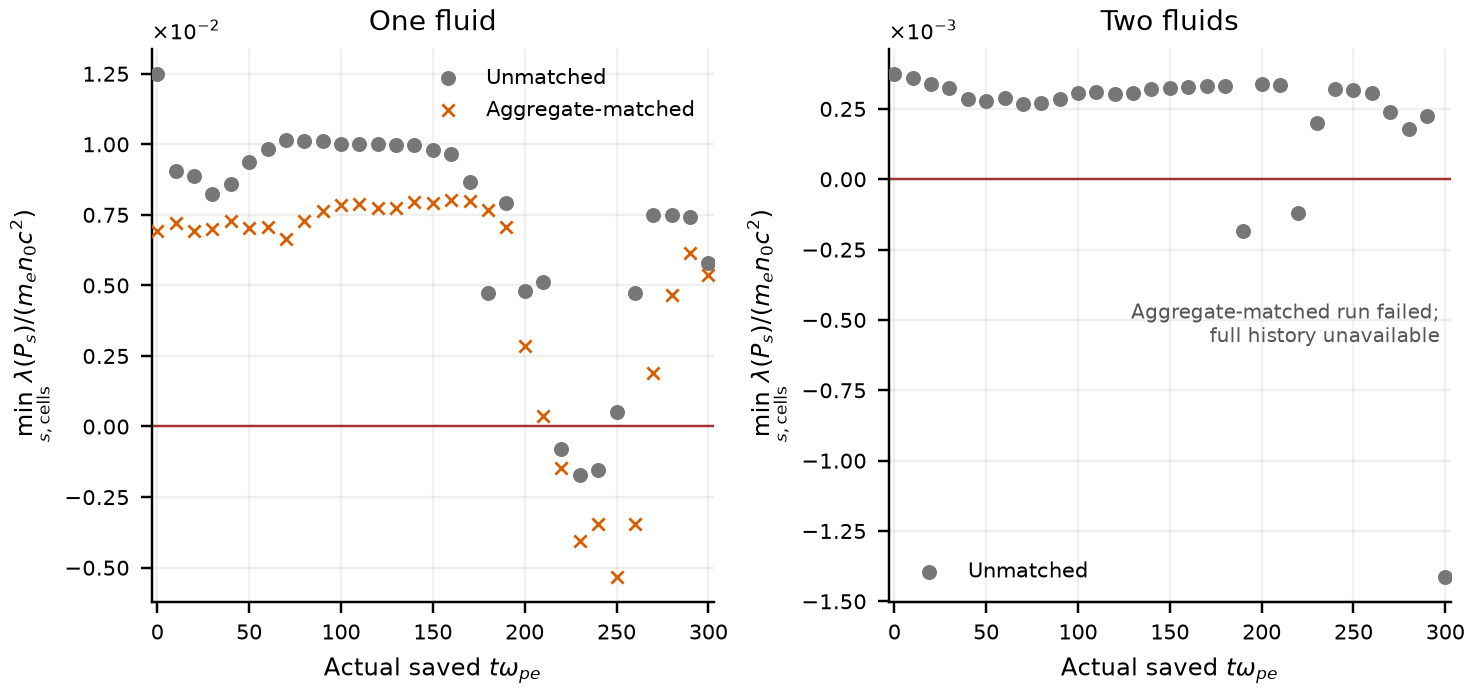
Figure 3. Smallest population covariance eigenvalue over all cells at each actual regular saved time for successfully completed runs. The failed matched two-fluid history is explicitly unavailable. Each point is a separate spatial minimum, not a tracked fluid parcel. The aggregate is not substituted for the population test. Negative points are non-realizable covariances. No connecting lines or interpolation are used, and unobserved timesteps are not certified by positive saved points. These are clean-source numerical cases, not the original archived trajectories.
3.4 Numerical endpoint sensitivity and baseline fidelity
The one-fluid unmatched and matched endpoints both pass the strict state checks and occur at exactly . Relative complete-grid errors against the same PIC reference change from to in density, to in , to in and to in . The changes are approximately , , and percentage points. They quantify the numerical endpoint response to the full aggregate-moment intervention; they are not current-only effects or validation of physical dynamics.
The clean one-fluid baseline differs from its archived source counterpart by , , and in the same respective field norms, at identical times. The maximum absolute density discrepancy is , so small global norms must not be read as uniform pointwise bounds. The exact original dirty implementation is not recovered. The two-fluid baseline’s population failure prevents a validated same-runtime two-fluid initialization pair; no such effect is inferred from a positive aggregate or from comparison with a different archived executable.
Table 3. Clean unmatched versus archived source-fluid output at eligible endpoints. Relative complete-grid differences are percentages, with the archived state as denominator. The final column is the combined norm of all eight stored field components, not an electromagnetic energy error. is the actual clean-minus-archived time. These norms are neither uniform pointwise bounds nor trajectory-admissibility certificates.
| Fluids | Stored fields | |||||
|---|---|---|---|---|---|---|
| One | 0 | 0.2104 | 0.7143 | 0.7158 | 1.2758 | 0.0695 |
Table 4. Numerical endpoint complete-grid relative errors (percent) against the archived PIC snapshot at . Every actual fluid output time is retained; no temporal interpolation is applied. Endpoint agreement does not validate a physical trajectory. Withheld entries are not zero errors.
| Case | Actual | ||||
|---|---|---|---|---|---|
| Archived source, one | 300.000150 | 3.973 | 28.340 | 36.357 | 34.577 |
| Archived source, two | 300.049985 | 2.648 | 21.736 | 34.261 | 31.522 |
| Clean baseline, one | 300.000150 | 3.976 | 28.305 | 36.287 | 34.656 |
| Clean baseline, two (withheld) | 300.043832 | — | — | — | — |
| Matched, one | 300.000150 | 3.477 | 26.512 | 28.855 | 30.772 |
| Matched, two (withheld) | — | — | — | — | — |
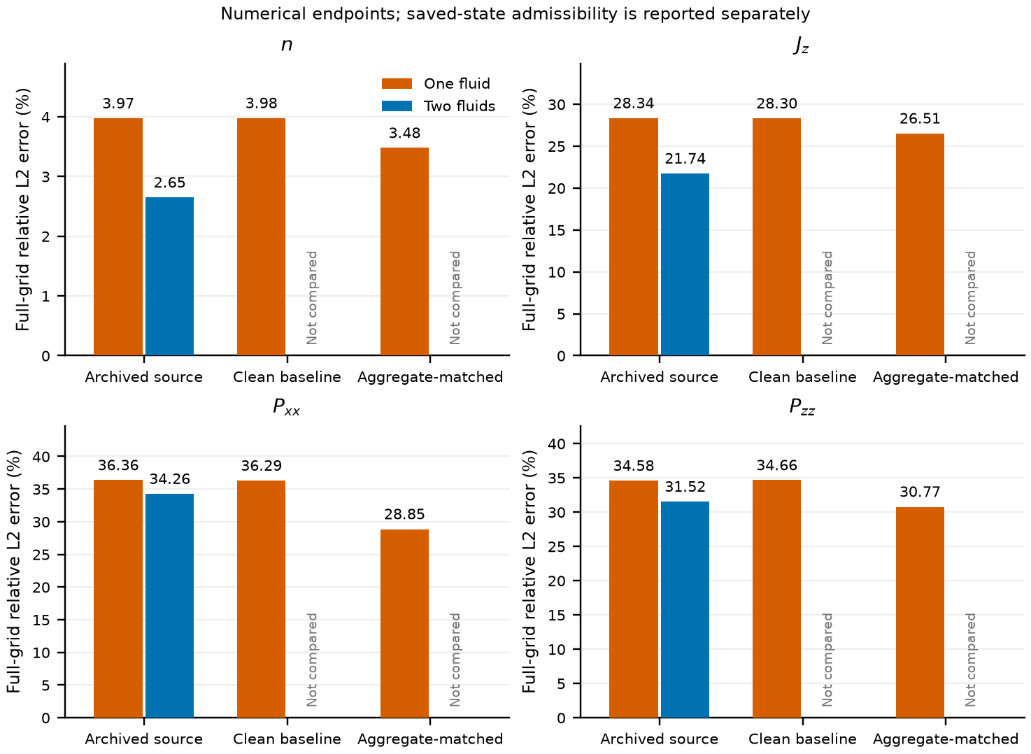
Figure 4. Complete-grid numerical endpoint errors against the same archived PIC reference. Withheld, nonconforming endpoints have no error bar; the annotation is not a zero error. Source archives supply context, while the same-runtime one-fluid pair isolates the specified initialization intervention at identical endpoint times. Its non-realizable saved histories preclude a physical-trajectory validation claim.
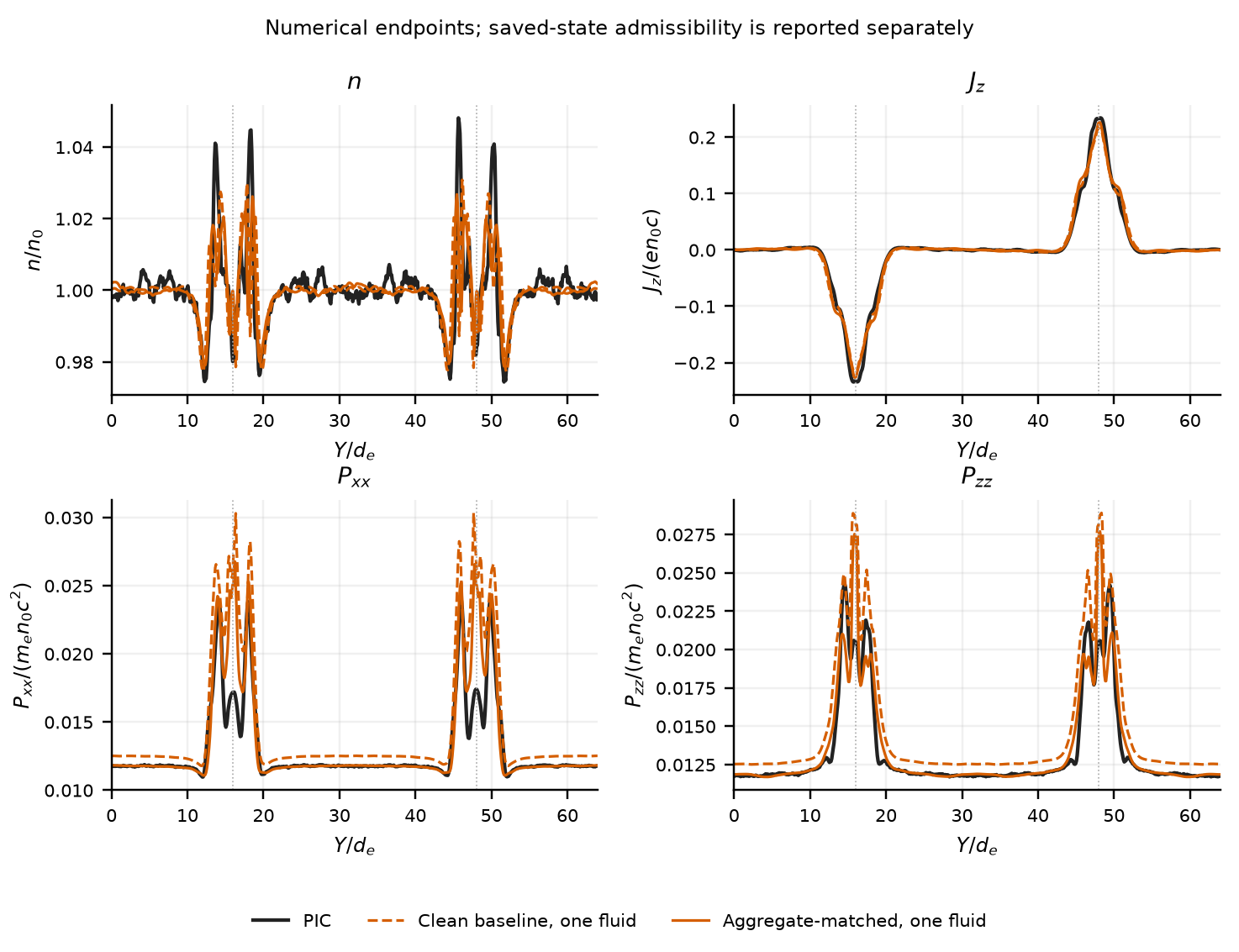
Figure 5. Full-domain, -averaged numerical endpoint profiles for eligible clean baseline and aggregate-matched cases, with the PIC reference. Missing curves are withheld cases, not vanishing fields. The projected profiles are distinct from the complete-grid norms in Figure 4. Positive endpoint covariances do not erase the saved intermediate failures.
The four terminal native outcomes, endpoint metric eligibility and saved-snapshot diagnoses remain separate in the accompanying machine-readable record: three normal native completions, one failed execution, three full saved-history scans and two eligible control endpoints. The failed run is not counted as a completed comparison or a 31-snapshot scan. No rejected endpoint receives primary performance metrics. The strict full-set comparison gate remains false when an endpoint is rejected; the explicit subset route reports numerical endpoints with history failures. The experiment uses one grid, one closure setting and one sampled initial target. There is no ensemble, resolution-convergence result, exact original executable recovery or physical causal bound. Lower endpoint errors and more saved covariance failures can coexist, as the one-fluid contrast demonstrates.
4 An auxiliary homogeneous linear-stability test
The source argues that its two-population description can capture linear growth of counter-streaming instabilities in reconnection [1]. Our calculation does not test those evolving distributions. It supplies a separate calibration example for the implemented local-isotropization closure: population drifts alone do not guarantee a correct collisionless kinetic spectrum. Closure-dependent differences in such spectra are established issues [7, 5]; the example below makes this validation issue explicit at the stated reference relaxation-rate scale.
Consider a homogeneous nonrelativistic electron plasma with immobile neutralizing ions. Two equal-density populations have ordinary velocities and isotropic thermal variance . Their longitudinal velocity marginal, normalized to unit density, is
A constant magnetic field parallel to leaves the longitudinal, gyrotropic perturbation subspace used below invariant. In the kinetic equation its gyrophase-rotation operator vanishes on gyrotropic perturbations; a longitudinal electric perturbation preserves that subspace. In the fluid equations, parallel velocity perturbations and a diagonal pressure perturbation with equal transverse entries have vanishing magnetic rotation terms. This justification concerns a uniform parallel field, not the source’s rotating field, transverse gradients or relativistic response.
The collisionless kinetic reference.
For , the only local minimum of is at zero. Indeed, , and is strictly concave on , with exactly one positive zero. The Penrose criterion [3] therefore tests
This integrand has a removable singularity at zero. At , . The alternating Dawson series has decreasing term magnitudes and gives the rational upper bound
Consequently , and this kinetic equilibrium has no exponentially growing longitudinal electrostatic mode for any real wavenumber. Direct quadrature gives ; the sign does not depend on that numerical evaluation.
Linearizing the finite-relaxation fluid model.
The source retains , with . Normalize the total plasma frequency, density, electron mass, charge magnitude and permittivity to one. For each beam , set , , and equilibrium diagonal pressure . Write its perturbations as , , and . For spatial factor , the invariant nine-variable system is
Here . A perturbation of multiplies the zero equilibrium deviator and thus contributes nothing at linear order, even when thermal speed is computed locally. Eliminating these variables independently, with temporal convention , gives
Proposition 4.1 (A finite-relaxation false positive).
At and , the collisionless kinetic equilibrium is stable to longitudinal electrostatic perturbations, while the local-isotropization fluid model is overstable for all sufficiently small positive .
Proof.
Kinetic stability follows from (7). At the longitudinal fluid pressure response has index three. Putting , , , its dispersion equation is
In units , its simple lower positive frequency is . Let and . Implicit differentiation of (9) yields
The sign can also be checked without the decimal value: the rational bounds make the numerator sum negative and the denominator sum positive. The root is simple, so its continuation has positive imaginary part for sufficiently small positive relaxation.
At a reference-scale rate obtained from and , , the matrix in (8) numerically gives
The eigen-equation, Gauss constraint , and independent dielectric residual are all below in the recorded checks; actual residuals are much smaller. The zero-relaxation matrix has no positive growth beyond roundoff. The literal fluid deck rounds its thermal speed to ; substituting the resulting also leaves positive growth, with a change smaller than . A periodic-box check using for , with , gives growth and a wavelength resolved by about 34 cells at the reported grid spacing. It is an -periodic mode of the homogeneous system, not a transverse eigenmode of the inhomogeneous current sheet.
These are continuum model diagnostics. They establish a false positive relative to the specified collisionless kinetic reference, including at the source’s positive relaxation-rate scale. They do not identify a mode measured in the original current sheet, replace a kinetic stability analysis of that sheet, or show that a particular nonlinear plot is contaminated. The source’s initial populations have a common velocity and its equilibrium varies across . No survival of this mode in that equilibrium is established. The benchmark is retained as an auxiliary closure test, rather than a counterexample to the source’s narrower application-specific capability claim.
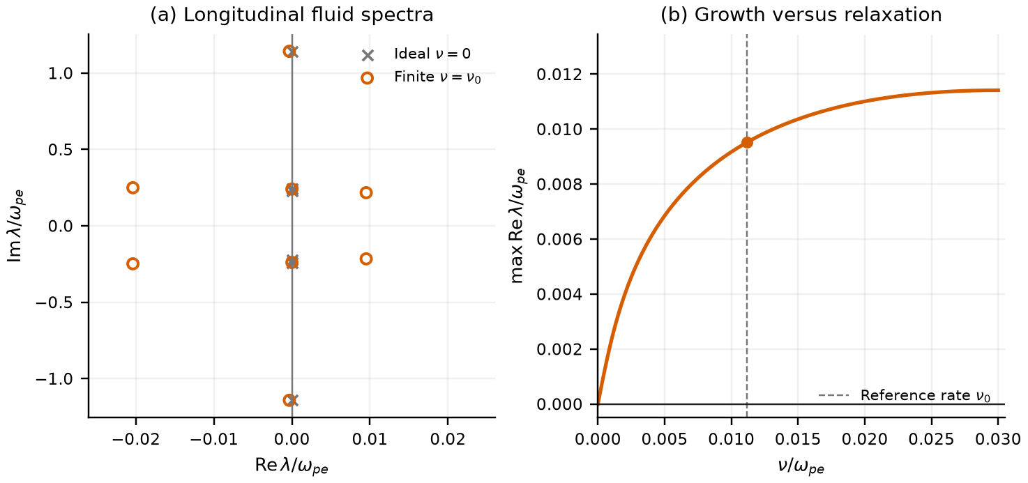
Figure 6. Homogeneous longitudinal test with and . Left: nonzero eigenvalues of the ideal and finite-rate fluid systems; the static Gauss-constraint mode is excluded. Right: the largest fluid growth rate as relaxation varies, with marked. The collisionless kinetic reference has no growing longitudinal electrostatic mode by the Penrose proof above. This comparison concerns the stated continuum closure, not an observed mode in the original reconnection calculation.
5 A secondary continuity clarification
On PDF p. 5, the source attributes its one-fluid density deficit to the vanishing of at the symmetric mid-plane, describing this as blocking transport into the sheet [1]. The value of a flux at one plane does not determine its divergence:
In particular, can be nonzero where . This is standard continuum kinematics, not a new plasma mechanism. Its role here is to qualify an explanation based on symmetry alone; the observed one-fluid density deficit and its dynamical cause remain separate questions.
Proposition 5.1 (A periodic density-accumulation example).
For , on a periodic coordinate ,
is a smooth positive solution of the one-dimensional continuity equation. Its total mass is , and while .
Proof.
The denominator is positive for every finite . Differentiating (14) gives directly. The standard integral , with and , gives the conserved mass. Evaluation at zero gives the stated increasing central density.
This is an exact kinematic transport example, not a self-consistent plasma–Maxwell solution or a substitute reconnection run. It refutes the inference from symmetry alone. The two-population model’s total density and density-weighted velocity obey exactly the same continuity equation after the population equations are summed. A one-fluid model loses the separate population-crossing information, but it is not geometrically forbidden from supplying or accumulating total density within a finite-width layer. Differences in the evolution of aggregate pressure and higher moments can still explain a particular benchmark failure.
6 Conditioning a relative heat-flux accuracy claim
The source’s Eqs. (3)–(4) and (B1)–(B2) are correct. For , put , , and . Recentring each population on the aggregate mean gives
The source explicitly defines the unnormalized three-term symmetrization, so its tensor formula has the required scalar factor three. Direct positive finite-mixture calculations, including nonunit mass, verify all entries.
For the scalar component and , define . Its counter-streaming contribution is
Thus the source’s cubic-drift explanation of the empirical parameter collapse requires qualification. Equation (16) also contains a temperature-contrast term linear in drift and can vanish by symmetry or cancellation.
Proposition 6.1 (A sufficient conditioned relative-error bound).
Suppose , with and stated nonnegative bounds . Set . If , then
Proof.
The exact residual is , so . The reverse triangle inequality gives . Division gives (17).
The bound is sufficient rather than necessary. Its imbalance/cancellation factor cannot be dropped. Equal population densities and temperatures give at any drift. With equal densities but unequal temperatures, , which is linear in drift.
A near-Maxwellian counterexample to a speed-ratio-only guarantee.
Let take values and with probabilities and . Then , and . For , let with a standard Gaussian. Let , with independent standard Gaussian transverse components, and define to have law , . It has zero mean, covariance , and third moment . Its total-variation distance from is at most . Give the populations equal densities and velocity laws
Each population density is a positive smooth Gaussian mixture, within in total variation of its matching Maxwellian. Their intrinsic temperature tensors are both , so , whereas . Consequently the relative closure error is one even when both and the thermal-to-beam speed ratio are arbitrarily small. The absolute residual does tend to zero relative to . The recorded calculations use and integrate the smooth laws with positive Gauss–Hermite quadrature.
This construction does not disprove the source’s measured collapse in its particular family of reconnection simulations. It identifies assumptions needed to extend that empirical observation to a relative-error guarantee. The source scan uses initial speeds; inserting those into a local bound would also require estimates of their subsequent evolution.
The valid limitation of a memoryless one-fluid closure.
Additional population information can be genuinely necessary. For example, let , and let each population be an isotropic Gaussian of variance . Choose a weight , set , and assign means and . For both and , the aggregate density is one, the mean is zero, and the pressure is . The respective values are zero and . Hence no arbitrary-distribution algebraic function of only can recover both third moments. This supports the source’s population-resolving motivation. It is not an impossibility statement for one-fluid descriptions with memory, extra variables, gradients or nonlocality.
7 Finite isotropization over a comparison interval
The source openly retains isotropization for numerical stability [1]. Its smallness relative to a fast local heat-flux scale does not establish closeness to zero-intrinsic-heat-flux evolution over an entire simulation. A homogeneous calculation makes the distinct finite-time parameter explicit.
At fixed density, let be a positive-definite pressure tensor and . The relaxation part alone satisfies
Its trace, and thus its thermal energy, are constant. For the Gaussian entropy diagnostic per particle, , one obtains
with equality only at isotropy. The inequality follows by applying the arithmetic–harmonic mean inequality to the three positive eigenvalues of . This is an entropy diagnostic of the moment model, not a measurement of PIC entropy or evidence of external heat input.
The deviation from the zero-relaxation homogeneous pressure is controlled by , not by alone. At the ideal reference-scale rate and ,
Thus an initially present homogeneous anisotropy would retain about of its amplitude over that interval. For the example at unit density, the entropy diagnostic increases by while the trace remains three.
This example does not establish how much relaxation changes the evolving source current sheet, whose anisotropy is time-dependent. It shows why a finite-duration sensitivity study in , or a direct comparison of the retained pressure-source terms, is needed when interpreting the implementation as approximately zero-heat-flux evolution. It does not dispute the source’s disclosed need for finite stabilization, nor identify irreversible adiabatic relaxation with external energy transfer.
8 Reproducible calculations and evidence limits
The repository separates reanalysis of archived simulation output from analytical model tests. The initial-state analysis uses the authors’ data dictionary, independently readable HDF5 attributes, published input decks, and explicitly aligned grid locations. The stability, continuity and moment calculations use specified equations and inputs and require no reconnection simulation executable.
The inspected Zenodo record is identified by the record-specific DOI 10.5281/zenodo.21114117; the source’s concept DOI is 10.5281/zenodo.21114116. Both resolve to this dataset family. The DOI agency lookup identifies DataCite, whose authoritative API record identifies the DOI as findable. A Crossref-only lookup returns no record; this is a registration-agency coverage difference. The direct repository link is https://zenodo.org/records/21114117. These identifiers do not denote two different simulations or a replacement data source.
Table 5. Selected verification outcomes. The code, data definitions and scope limits distinguish initial-state reanalysis from independent continuum tests.
| Check | Outcome |
|---|---|
| Initial moment current at | 11.5309% below staggered curl |
| Initial at that row | 0.615446655 |
| Exact mixture identities | All scalar and tensor checks pass |
| Symmetry-plane continuity | Zero normal velocity; increasing density |
| Conditioned relative-error example | 0.024134 0.036243 |
| Identical one-fluid lower moments | Different third moments |
| Finite-relaxation mode growth | |
| Homogeneous relaxation over | 3.4941% anisotropy remains |
The initial analysis used selected ZIP members from the public Zenodo archives, with bounded partial responses, member lengths, CRC32 and SHA-256 checks. The final revision additionally retrieved all three complete source ZIPs, totaling 1,367,080,859 bytes. Each full byte count and publisher-declared MD5 matches; a full SHA-256 was also computed and recorded. All 13 original PIC HDF5 and five initial fluid BP inputs were then read by exact name from those verified complete ZIPs and matched to their earlier member hashes. The portable whole-archive receipt supplements the retained historical selective-retrieval records; it does not silently change the analyzed inputs. Small derived profiles and provenance are included with attribution. The original paper and full simulation archives are not redistributed here.
Numerical checks preserve the exact mixture identities rather than treating them as errors. The linear calculation is checked independently through an eliminated dielectric relation and the Gauss constraint, in addition to the matrix eigenvalue residual. The kinetic comparison has an exact rational stability bound, so its conclusion does not depend on locating a numerical threshold near marginal stability. The continuity example satisfies the transport equation explicitly. These checks test the scientific statements used in the paper, not only whether a plotting script runs.
The execution record in Appendix B pins the code, input hashes, numerical results and environment. Its timestamps are author-environment execution evidence, not third-party certification or independent human peer review. The accompanying verification script reports actual failures instead of silently replacing absent inputs with synthetic data.
New clean-source Gkeyll evolutions and their endpoint/history checks are reported in Section 3. No new OSIRIS simulation was run. The published input decks and archived diagnostics do not uniquely identify the authors’ exact executable builds. In particular, the documented custom velocity diagnostics are interpreted using the authors’ explicit data dictionary; we do not assert that a present public source checkout is the private build that produced them. This limits claims about implementation internals while leaving the documented archived-moment comparison testable. The new numerical contrasts are conditional on the identified clean runtime; saved pressure failures are retained rather than clipped, masked or repaired.
9 Consequences for controlled validation
An initialization audit should precede attributing every later difference to the heat-flux closure. The current test exposes a mismatch in physical moments despite matching algebraic drift expressions. A controlled repeat should match density, ordinary mean velocity and the selected pressure definition, and report the initial magnetic curl and moment current on their actual staggered locations. If relativistic particle initialization and a nonrelativistic fluid model are compared, the conversion and the target moment convention must be stated explicitly. The cold proper-velocity conversion alone is not a proof that finite-temperature moments have been matched.
The clean one-fluid endpoint contrast establishes a numerical response to the aggregate-moment intervention: all four tested endpoint errors decrease. It does not establish a physical cause of the source’s reconnection differences. The intervention replaces the conserved moment vector through second order, including sampled spatial variation; it is not confined to the mean current. Both one-fluid saved histories have covariance failures, the clean unmatched two-fluid endpoint is rejected, and the matched two-fluid run fails before producing its comparison endpoint. A smaller endpoint error cannot erase those failures or substitute for realizability and resolution checks. We therefore do not infer that correcting the drift eliminates the reported density deficit, reproduces full PIC heat flux with one fluid, or reverses the source’s physical conclusion.
The archived one- and two-fluid endpoints remain positive definite under the same tensor test. This distinguishes an observed failure of the identified clean implementation from a claim about the unavailable dirty executable. The finite snapshot archive does not establish that the original intermediate trajectory was admissible, either. Identified executable provenance, full-tensor state checks and grid-converged controls are needed before transferring the numerical endpoint changes into a physical causal statement.
The auxiliary homogeneous stability test supplies a separate calibration. Retaining population drift creates the possibility of streaming modes; it does not ensure the correct kinetic susceptibility or growth rate. The implemented relaxation should be included in the dispersion calculation. Finite relaxation can change a spectrum even when the unperturbed pressure is isotropic and the relaxation source vanishes at equilibrium. In the stated example the resulting growing mode is a false positive relative to the collisionless kinetic reference. This is a test of a model’s continuum response, not evidence that the original simulation visibly contains that mode. The new clean-source evolutions do not provide a source-sheet eigenanalysis or a physically validated, grid-converged matched comparison. This diagnostic comment quantifies numerical sensitivity and exposes validation requirements; the source’s nonlinear physical conclusions are not thereby disproved.
The pressure-source diagnostic should also distinguish a third-moment amplitude from its divergence. The scale proxy used in the source is a useful estimate when is an appropriate gradient length. It is not identical to . A spatially constant nonzero heat-flux tensor has a finite amplitude proxy and zero divergence. The source explicitly notes that its isotropization closure constrains a divergence and omits the reconstructed fluid tensor from some plots; we do not characterize that disclosure as a hidden omission. Direct source-term comparisons and rate convergence would make the approximation more informative.
Finally, the source’s time-maximum spatial score is a best-time diagnostic, not a uniform-in-time error bound or a forward prediction test at every scan point. The conditioned estimate above explains why both absolute residuals and a nondegenerate denominator are needed when assessing relative accuracy. These qualifications preserve the observed scan and suggest measurements needed before extending its interpretation to new current sheets, later island recirculation, or turbulence.
The valid component-to-aggregate moment decomposition remains the foundation of this analysis. Additional labels carry information absent from a generic state described only by total density, velocity and pressure. The corrections identify controls and assumptions needed for using that additional information reliably, rather than a general rejection of multicomponent fluid modeling.
10 Conclusion
Matching nominal drift expressions does not ensure matched moments between a proper-momentum PIC initialization and an ordinary-velocity fluid initialization. The archived PIC moments and reloaded fluid output make that distinction quantitatively testable. The full-profile and conditional finite-temperature checks strengthen that initial-state finding. Clean-source evolutions quantify numerical endpoint sensitivity, but saved covariance failures prevent interpreting lower endpoint errors as validation of a physical trajectory. The separate homogeneous benchmark shows why finite isotropization should be calibrated as part of a closure; it establishes no unstable eigenmode of the source’s inhomogeneous sheet. The exact moment decomposition remains valid and useful. Matching aggregate moments, checking the complete pressure tensor, identifying the executed code, and testing resolution are distinct requirements. The original archived endpoint population tensors pass the covariance test; failures in the identified clean implementation do not establish failures in the unavailable dirty build. Correcting the density-transport explanation and conditioning relative-error statements supports further comparison without declaring the source’s nonlinear physical conclusions disproved.
Author and methods disclosure
Taylor Kalin is the author and is responsible for this study. OpenAI Codex assisted with source inspection, derivations, code, data analysis, and manuscript preparation under his direction. Separate AI-agent checks were used during preparation; they are not represented as independent human expert review. Reported results combine deterministic classical calculations, reanalysis of public archived moments and new clean-source fluid evolutions. No new PIC simulation or experimental measurement is claimed. Numerical endpoint comparisons and saved-state admissibility diagnoses are reported separately.
Funding and competing interests.
This study was self-funded by Taylor Kalin, including computing resources and AI tools. No external funding was received. No competing interests were reported for this study.
Prior dissemination and review sequencing
This is one study. GitHub and AiraXiv deposits are preprint versions of the same work. Agent-only editions, where used, identify Taylor Kalin as canonical author and human operator; they are not independent new findings. Review venues are sequenced to avoid concurrent consideration of the same manuscript. Actual identifiers and outcomes are recorded at https://github.com/Teylersf/counterstreaming-heatflux-audit in the publication-status record.
References
[1] Madox C. McGrae-Menge, Jacob R. Pierce, Maria Almanza, Alexander Velberg, Nathaniel Barbour, William D. Dorland, Nuno F. Loureiro, Frederico Fiuza, and E. Paulo Alves. Counter-streaming heat-flux closure for electron-only collisionless magnetic reconnection, 2026. Audited version 1, submitted 8 July 2026. https://arxiv.org/abs/2607.07106v1.
[2] Madox McGrae-Menge. Counter-streaming heat-flux closure for electron-only collisionless magnetic reconnection. Zenodo, record 21114117, July 2026. Published 2 July 2026. DataCite record DOI: 10.5281/zenodo.21114117; concept DOI: 10.5281/zenodo.21114116. Input decks and archived diagnostics. https://zenodo.org/records/21114117.
[3] Oliver Penrose. Electrostatic instabilities of a uniform non-Maxwellian plasma. The Physics of Fluids, 3(2):258–265, 1960. https://doi.org/10.1063/1.1706024.
[4] Gregory W. Hammett and Francis W. Perkins. Fluid moment models for Landau damping with application to the ion-temperature-gradient instability. Physical Review Letters, 64(25):3019–3022, 1990. https://doi.org/10.1103/PhysRevLett.64.3019.
[5] Liang Wang, Ammar H. Hakim, A. Bhattacharjee, and K. Germaschewski. Comparison of multi-fluid moment models with particle-in-cell simulations of collisionless magnetic reconnection. Physics of Plasmas, 22(1):012108, 2015. https://doi.org/10.1063/1.4906063.
[6] M. V. Goldman, D. L. Newman, J. P. Eastwood, and G. Lapenta. Multibeam energy moments of multibeam particle velocity distributions. Journal of Geophysical Research: Space Physics, 125(12):e2020JA028340, 2020. https://doi.org/10.1029/2020JA028340.
[7] Jonathan Ng, Ammar Hakim, J. Juno, and A. Bhattacharjee. Drift instabilities in thin current sheets using a two-fluid model with pressure tensor effects. Journal of Geophysical Research: Space Physics, 124(5):3331–3346, 2019. https://doi.org/10.1029/2018JA026313.
[8] Emil R. Ingelsten, Madox C. McGrae-Menge, E. Paulo Alves, and Istvan Pusztai. Data-driven discovery of a heat flux closure for electrostatic plasma phenomena. Journal of Plasma Physics, 91(2):E64, 2025. https://doi.org/10.1017/S0022377825000285.
[9] Emil R. Ingelsten, Madox C. McGrae-Menge, E. Paulo Alves, and Istvan Pusztai. Data-driven multi-species heat flux closures for two-stream-unstable plasmas with nonlinear sparse regression. Physics of Plasmas, 33(4):042106, 2026. https://doi.org/10.1063/5.0311956.
[10] OSIRIS Collaboration. Momentum distribution: udist. OSIRIS Reference Guide. https://osiris-code.github.io/osiris/reference/udist. Accessed 28 October 2026; current public documentation, not identification of the original simulation build.
[11] OSIRIS Collaboration. OSIRIS momentum-distribution and particle-loading source code. Public source, commit a858fe1da3d6dbf3652b16556af87f7dad7881eb. Accessed 28 October 2026. Conditional loader interpretation; not identification of the original executable. https://github.com/osiris-code/osiris/tree/a858fe1da3d6dbf3652b16556af87f7dad7881eb/source/spec.
[12] Gkeyll Project. The eigensystem of the ten-moment equations written in conservative form. Gkeyll developer documentation. Accessed 28 October 2026; explicit ten-component conserved-vector layout. https://gkeyll.readthedocs.io/en/latest/dev/tenmom-eigensystem.html.
A Source passages and artifact scope
All source equation and page locators refer to the PDF of arXiv:2607.07106v1 [1]. The supplied ten-page PDF is byte-identical to a fresh versioned arXiv download: 7,847,791 bytes, SHA-256
fc5344e2ba8f4db98baf90d805bb6b7ce8835c32ea7bf54bba4d62f405b955a3.
The official history checked on 28 October 2026 lists v1 submitted 8 July 2026 at 07:43:25 UTC, with no later revision or journal reference. The PDF displays 9 July; the experimental HTML displays 24 August. The original apssamp.tex, line 95, uses \date{\today}, so separately compiled display dates are not version identifiers. No source author has been contacted, and no author confirmation is claimed.
The separately retrieved versioned source archive has 7,439,982 bytes and SHA-256
4f9abd5f41ffca0f1879981429165ff1a989276792c812e860f57cb5038c3b2e.
The repository’s selective excerpts contain six attributed files and 17 fragments, with original TeX line and character positions. A standalone verifier checks the archive and source hashes and reconstructs every excerpt without executing the source or making network requests. The full PDF and source archive are not redistributed.
The stated initialization.
Appendix A, p. 6, states that the electron fluid velocities are initialized from
Appendix C, p. 8, states that the fluid simulations inherit the PIC domain, grid, boundary conditions and magnetic-field initial condition exactly. It specifies the common initial drift
and thermal speed for the electron fluids. These are the matching statements tested in the main text. Original TeX locators are lines 225, 244 and 280; the printed seed is Eq. (A3), lines 238–240.
The current public udist documentation describes ufl and spatial_ufl as fluid momentum in proper-velocity units and gives relativistic momentum addition as the default [10]. This documents the input-language interpretation; it does not identify the authors’ exact historical executable. For the archived diagnostics, the definition used here comes directly from the authors’ Zenodo deposit description [2]:
The deck and diagnostic checks, rather than an assumed private code revision, support the initial-moment comparison.
The density-transport explanation.
The main text, p. 5, attributes the one-electron-fluid density deficit to the following mechanism:
“at the mid-plane by symmetry, blocking 1-e-Fluid transport into the sheet”.
The complete argument is in original TeX line 191. The symmetry-plane continuity calculation assesses this causal explanation; the plotted density deficit remains empirical evidence from the reported benchmark.
The implemented closure and instability claim.
On p. 4 the source specifies the finite local model
with an isotropization timescale of about (original TeX line 179). Figure 3’s caption, p. 4, explicitly omits its contribution from the displayed fluid heat flux and notes that only its divergence is constrained (line 166). The finite term is therefore a disclosed part of the model. The longitudinal calculation in this study tests that finite model, rather than silently replacing it by its zero-coefficient limit. On p. 5 the source also asserts that the two-electron-fluid model can capture linear growth because the instabilities are due to counter-streaming (line 207). The general importance of closure choice for instability fidelity is established prior context [7].
Accuracy metric and retained qualifications.
The color in source Fig. 4, p. 5, is the best-time score
(original TeX line 198). Its proposed thermal/drift scaling is explained in line 202. The present audit distinguishes this empirical best-time diagnostic from a uniform error guarantee; it does not claim to have rerun the parameter scan. The source acknowledges later stream folding (p. 5, line 207), separate fluid color scales and amplitude differences in the full-tensor comparison (Fig. 5, p. 7, line 250), and kinetic free-expansion limitations (Appendix C, p. 8, line 293). The exact mixture identities in source Eqs. (3)–(4) and (B1)–(B2) are preserved as valid algebra.
B Pinned execution record
The following immutable commit pins the checked code, input decks and evidence files:
Every source/input/evidence hash listed in the inventories was checked against that commit. The inventories and manuscript files generated afterward are derived release outputs.
Historical original verification.
The original eight-group execution below retains its original timestamp, environment and results. Its four numerical code files are byte-identical at the pinned commit. This does not assert that every later analysis was executed together in that historical run.
Started UTC: 2026-10-28T23:09:06.987425+00:00
Python: 3.12.14 (main, Aug 25 2026, 14:01:42) [MSC v.1944 64 bit (AMD64)]
NumPy: 2.3.5
h5py: 3.16.0
PASS: initial_current
PASS: initial_pressure
PASS: mixture_identities
PASS: continuity_symmetry
PASS: conditioning_counterexample
PASS: singlefluid_nonidentifiability
PASS: finite_relaxation_stability
PASS: isotropization_entropy
All assertions passed: true
Exit status: 0
The selected verification table is unchanged from this original eight-group record.
Reproduction and later analyses.
git clone https://github.com/Teylersf/counterstreaming-heatflux-audit.git
cd counterstreaming-heatflux-audit
git checkout b47a51608726b80931fc607f0f44a02ab4bfbfdd
python -m pip install -r requirements.txt
python experiments/fetch_data.py
python experiments/data_checks.py
python -X utf8 experiments/verify.py
python -X utf8 experiments/make_figures.py
python experiments/profile_sensitivity.py
python experiments/revision_data.py --inventory --fetch
# Separate Linux ADIOS2 reader environment:
python experiments/revision_data.py --decode-bp
python experiments/revision_data.py --compare
python experiments/thermal_loading.py
The pin additionally covers the portable full-PIC moment exporter, BP reader, matched-input preparer/initializer, native control runner, completed-output collector and comparison analyzer. Their CLI help and the data documentation specify the required cache paths and immutable run pins; the code itself does not imply that an uncompleted case was measured. The three complete source ZIP archives passed byte-size and publisher-MD5 checks, with full SHA-256 hashes and selected-member bindings recorded in data/full-archive-verification.json. The native runs retain their recorded launch-code revision fba895a3989b0855186b38c2e77d8c9d23aac94c; the final evidence pin above additionally contains the later analysis outputs. The supplied result lists 2 control-case endpoint comparisons and 2 accepted endpoint-decoding receipts. The all-four completed-and-compared flag remains false; pending or rejected cases remain explicit in the pinned inventories.
Native outcomes, endpoint eligibility and saved histories.
The separate admissibility record retains all four native outcomes: 3 normal regular30 completions, 1 terminal execution failures, and 1 endpoints rejected by the strict state guard in the supplied evidence. Native completion and positive-definite endpoint eligibility are separate facts. Rejected endpoints have no accepted primary comparison metrics. The failed native cases are matched_two_fluid. They supply no accepted regular30 endpoint or comparison metrics. Their pressure histories are explicitly unavailable; no regular0–30 scan is inferred from the available earlier outputs. matched_two_fluid: its last closed regular output is frame 22 at . The exact native/portable receipt and console hashes are retained with the selected independent failure proof. This scalar observation does not identify the failing transient, species or update time. The rejected endpoint cases are baseline_two_fluid. The bound endpoint-admissible NUMERICAL sensitivity pairs are one_fluid_initialization_effect. Each retains its exact runtime, native/portable receipt hashes, actual endpoint times and clean-base versus archived-source check. These endpoint contrasts do not establish physical causality, convergence or valid dynamics. baseline_one_fluid: the saved-state covariance test fails at regular frames 22, 23, 24. These history failures remain attached to any eligible endpoint contrast. baseline_two_fluid: the saved-state covariance test fails at regular frames 19, 22, 30. These history failures remain attached to any eligible endpoint contrast. matched_one_fluid: the saved-state covariance test fails at regular frames 22, 23, 24, 25, 26. These history failures remain attached to any eligible endpoint contrast. matched_two_fluid: its regular0–30 pressure-history diagnostic is unavailable following terminal native failure. Saved snapshots do not certify the intervening timesteps, locate the first invalid update, or identify the operator that produced a loss of admissibility. No state was clipped or repaired. Third-diagnostic normalization qualifications remain attached to the heat-flux comparisons. No native deposited-current comparison or inhomogeneous-sheet eigenanalysis is claimed.
Compact file record.
The complete code hashes are grouped in code-pin.json; the separate output manifest groups revision results, supporting evidence and optional final control records. Only these fixed summary rows are repeated here, so a larger evidence inventory does not lengthen the PDF hash table.
| File | SHA-256 |
|---|---|
results/verification.json | 6e724e564d4ca23bf718d4add4eded9311aa6ebbeb161c4abc606ec750f01491 |
results/code-pin.json | 4d85d5c0aed7f7cf7f0495e08ab1189d19d51f0ea51e4912277d863ce72d95b0 |
results/execution-output-manifest.json | 55a9c92b3b9c7ca0b099e19ba794c145da54fe2108790ed8bd346eccb7a87a7f |
This is an author-environment execution record, not third-party certification or independent human peer review.