Abstract
We audit arXiv:2508.15691v2 and the published Quantum Science and Technology article *Trotter-based quantum algorithm for solving transport equations with exponentially fewer time-steps* by Zylberman, Fredon, Loureiro and Debbasch. Ten registered correction groups persist in the directly inspected journal PDF. Exact counterexamples refute conservation of spatial derivative norms for variable transport fields and the signed-overlap identity assigned to a controlled-SWAP circuit. Further corrections concern transport and Liouville signs, Fourier inversion, moment normalization, constants and index ranges. We retain finite-time regularity factors and apply established commutator reasoning to obtain a coefficient-aware finite-grid operator bound proportional to inverse mesh spacing rather than its square for smooth periodic coefficients. This sharpens the chosen comparison baseline without proving a complete repaired vector-norm theorem or disproving the usefulness of smooth-state analysis. Independent calculations reproduce the reported eight-point discretization errors and a separate periodic splitting diagnostic. A version concordance, attributed source statements and numerical provenance tables make the findings directly checkable. The journal's added Gaussian-width, circuit-cost and boundary qualifications are acknowledged. No end-to-end quantum advantage, general impossibility result or inference about unavailable implementation code is claimed.
Editorial notes
Points the editor recorded on accepting the paper. They are published with the article; the authors were not required to address them before publication.
- Section 7 cites only submissions/zenodo-doi-verification.json, whereas the round-3 response letter names submissions/zenodo-doi-verification-round2.json as the current receipt, so list the round-2 receipt in Section 7 as well.
- Section 7 should state the DataCite registration date of DOI 10.5281/zenodo.23770769 so readers can reconcile it with the earlier unresolved registry lookups.
- The Abstract is printed twice (before the body and again as the body's '## Abstract' section); remove the duplicate in the typeset version.
- The 'Preprint and review disclosure' paragraph in Section 7 describes venue sequencing policies that are not part of the scientific record; condense it to a one-line preprint disclosure.
Corrections and resource bounds for the Trotter quantum transport algorithm
Taylor Kalin
Independent researcher; https://taylorkalin.com
ORCID: 0009-0003-9000-9315; correspondence: teylersf@gmail.com Version 1.1.1; 29 October 2026
Abstract
We audit arXiv:2508.15691v2 and the published Quantum Science and Technology article Trotter-based quantum algorithm for solving transport equations with exponentially fewer time-steps by Zylberman, Fredon, Loureiro and Debbasch. Ten registered correction groups persist in the directly inspected journal PDF. Exact counterexamples refute conservation of spatial derivative norms for variable transport fields and the signed-overlap identity assigned to a controlled-SWAP circuit. Further corrections concern transport and Liouville signs, Fourier inversion, moment normalization, constants and index ranges. We retain finite-time regularity factors and apply established commutator reasoning to obtain a coefficient-aware finite-grid operator bound proportional to inverse mesh spacing rather than its square for smooth periodic coefficients. This sharpens the chosen comparison baseline without proving a complete repaired vector-norm theorem or disproving the usefulness of smooth-state analysis. Independent calculations reproduce the reported eight-point discretization errors and a separate periodic splitting diagnostic. A version concordance, attributed source statements and numerical provenance tables make the findings directly checkable. The journal's added Gaussian-width, circuit-cost and boundary qualifications are acknowledged. No end-to-end quantum advantage, general impossibility result or inference about unavailable implementation code is claimed.
1. Introduction
Encoding a discretized transport solution in quantum amplitudes can reduce the number of memory qubits dramatically. The remaining questions concern how that state is prepared, how accurately it evolves, what measurements return, and what resources each of these operations consumes. A statement about a time discretization bound answers only one of those questions. It should be judged on its own assumptions before being interpreted as a computational advantage over a classical solver.
The audited preprint [1] studies periodic transport with a velocity field whose component in each coordinate direction is independent of that same coordinate. It combines centered finite differences, quantum Fourier transforms and first-order product formulas. Its central analytical observation is sensible: an operator containing an increasingly fine discrete derivative can have a large worst-case norm while acting moderately on a fixed, smooth function. The paper compares a vector-dependent error estimate with a crude product of operator norms and reports an exponential reduction in the predicted number of steps as the number of qubits per coordinate grows.
Several details require correction before this conclusion can be used reliably. Smoothness is preserved for a finite time under a smooth transport flow, but its derivative norms need not retain their initial values. Two separately prepared states do not supply a phase reference through a SWAP test. A sign convention for a shift acting on ket labels has the opposite action on its amplitude array. These issues are algebraic and can be checked without access to a quantum computer. They are also distinct from whether the program unavailable in the inspected arXiv materials used the printed expressions literally.
This paper has three purposes. First, we identify reproducible failures in specified equations of the supplied edition. Second, we replace the incorrect derivative conservation argument and improve the operator-norm baseline using the structure of finite differences. Third, we delimit what survives: unitary directional transport, the practical benefit of smooth-state estimates, and the reported small-grid error magnitudes. This separation prevents a transcription error from being mistaken for a general impossibility result and prevents a valid numerical illustration from repairing an invalid proof step automatically.
Our contribution is a technical correction comment, not an authorized revision of the original authors' paper. The article appeared in Quantum Science and Technology 11, 025015 (2026), DOI 10.1088/2058-9565/ae488e [2]. Initial requests encountered a publisher challenge; a later ordinary publisher PDF request succeeded. We then directly inspected the journal text and verified that all ten correction groups registered for the supplied arXiv edition persist, with renumbered appendix equations. Section 3.1 reports the version concordance. The journal also adds substantive qualifications, which this revision credits rather than treating the two editions as identical.
2. Related work and mathematical setting
An, Fang and Lin [3] established the usefulness of vector-norm analysis for time-dependent Hamiltonian simulation with unbounded operators. Their treatment includes an unbounded kinetic operator and a bounded potential under stated commutator assumptions. The audited paper acknowledges that antecedent and addresses a different transport decomposition. Our counterexamples do not dispute the earlier theorem, nor do they establish that the transport paper has no new analytical content. They address specific claims in its extension and the interpretation of its comparison baseline.
The controlled-SWAP identity is established in the quantum fingerprinting literature [4]. Hadamard tests and quantum amplitude estimation [5] can estimate other quantities with suitable controlled preparation and access assumptions. These protocols are not interchangeable solely because each produces a scalar measurement. In particular, retaining a phase reference through a controlled preparation differs physically from comparing two independently prepared state registers.
Commutator-sensitive product-formula estimates are established theory [6]. Our Section 4.2 is an explicit application to finite-grid transport, not a new general splitting theorem. Burgarth et al. [9, Theorem 2] further show that the commutator on an initial state cannot universally certify finite-time error. Their stationary exact-trajectory example also rules out replacing it solely by its maximum along the exact trajectory. Actual defects involve intermediate split trajectories or additional product and remainder controls. Our initial-state commutator diagnostics therefore accompany independently calculated evolution errors; they are not error certificates. A separate contribution by the four transport authors treats anisotropic diffusion and convection [10]. Its arXiv v1 and Springer proceedings version are separately identified; this audit does not automatically establish any correction to that proceedings article.
Throughout, the spatial domain is the unit torus, with smooth periodic real velocity , and
We adopt the original componentwise condition when discussing its directional implementation. This implies , so the continuum flow preserves volume and the solution's norm. It is stronger than divergence freedom. Unless stated otherwise, dimension, finite-difference order, final time and continuum input functions remain fixed while the grid is refined. Constants may depend on all of those fixed quantities.
Let , , and be the centered first-derivative coefficients of order , with for . We distinguish a forward ket shift from a forward amplitude translation . They are inverse conventions. The consistent amplitude derivative used below is
The Hermitian transport Hamiltonian corresponding to (1) is , because . Here is the diagonal matrix of samples of . Under the componentwise condition, and commute. This sign convention will be kept explicit in every test.
3. Methodology and evidence boundary
The supplied PDF has 34 pages, 4,798,118 bytes and SHA-256 8c3e5bf0c6c063bb96f383066c8a5640659e6a69a40a4d990e90901dd56d0fd2. It is byte-identical to the official versioned arXiv v2 PDF. We read its full text and appendices, inspected displayed equations, and compared them against the official TeX archive [1]. We also read the full journal PDF [2] and visually verified the disputed formulas. The arXiv archive contains manuscript, bibliography and figure images, but not the original study's simulation programs or raw hardware outcomes. The journal supplies a data-availability statement; we did not obtain executable author code or a hardware job record. These are evidence-specific statements, not a claim that no code exists anywhere. Unless a journal locator is explicitly given, source equation/page references in Sections 4-5 retain arXiv v2 numbering; Section 3.1 and Appendix A provide their journal concordance and source statements.
We use two independent calculation scripts. experiments/reproduce.py generates analytical counterexample samples, finite-matrix checks, five CSV tables and three figures. experiments/resource_counterchecks.py independently checks the main measurement and convention examples, reproduces the reported hardware-discretization error magnitudes, and evolves a separate smooth periodic transport problem. Both use double-precision NumPy; Matplotlib is required only for the first script's figures. There is no fitting to experimental data, stochastic selection of favorable runs, or use of a local language model as a numerical oracle. The calculations use CPU arrays; releasing GPU memory is not a condition for these small checks.
We classify evidence at three levels. A literal equation failure is demonstrated by substitution or a finite matrix whose result contradicts the printed statement. A resource qualification identifies parameters hidden when an asymptotic assertion fixes an input family. An implementation uncertainty identifies what cannot be inferred from manuscript formulas without the actual program or data. The first level justifies correction; the second justifies narrower wording; the third justifies restraint rather than an accusation.
The main numerical tolerances are for analytic shear quadrature and for elementary SWAP identities. The translation test refines from 16 to 128. The commutator test uses per coordinate, exploiting a tensor factorization to evaluate the exact operator norm using only -dimensional matrices. For the separate periodic evolution diagnostic, a 2,048-step Strang reference is compared with a 1,024-step reference to quantify reference error. That difference is reported alongside the first-order splitting error rather than assumed negligible silently.
The repository supplies source provenance, a correction registry, numerical outputs, environment versions, and a hash manifest. Appendix A quotes the audited statements and reproduces their equations with attribution. Appendix B defines the norms, gives matrix constructions, and tabulates numerical provenance within the paper. The tests are deliberately small and falsifiable. They verify algebra and illustrate limiting behavior; they are not a hardware replication, an assessment of fault-tolerant gate counts, or a benchmark against an optimized classical PDE code. Journal conclusions now rest on its downloaded text and rendered formulas, not metadata or indexed snippets.
3.1. Journal edition and statement concordance
The version comparison now includes the published article [2] as well as the previously audited arXiv:2508.15691v2 [1]. The official publisher PDF was obtained through an unauthenticated request initiated on 29 October 2026 at 15:57:49 UTC; it is available through the PDF download action on the article's DOI landing page. It has 2,014,929 bytes and SHA-256 1b8f24ed2bcd4979526977581fc795f80d90a6efeacfbe28e65339cf8b4803e1. Its 34 PDF pages comprise an unnumbered publisher cover followed by printed article pages 1-33. The article identifies its publication as Quantum Science and Technology 11, 025015, DOI 10.1088/2058-9565/ae488e, published 3 March 2026 under CC BY 4.0. The title, four authors, DOI, dates and license were checked on its first printed page.
Version 1 of this audit accurately recorded the access challenges encountered in its available sessions and restricted its conclusions to the supplied preprint. The subsequent successful retrieval makes a direct journal comparison possible. The comparison below uses the downloaded PDF, extracted text and direct inspection of the relevant rendered formulas. Its conclusions do not rely on the publisher's open-access label or search-index excerpts. The public machine-readable record is data/journal-comparison.json.
The table retains the correction IDs used in the original registry. An arXiv page is the page printed in that preprint; a journal page is the printed article page, followed by its one-based PDF page in parentheses. Journal equation numbering is given as printed. The status persists means the specified printed discrepancy remains in this obtained journal edition. It does not establish which formulas were used in the authors' unavailable implementation code or how the published figures were generated.
| ID | arXiv v2 locator | Journal locator: printed page (PDF page), label | Status | Description |
|---|---|---|---|---|
| C1 | p.12, paragraph after Theorem III.4 and footnote 10; p.29, Appendix B opening | p.11 (12), paragraph after Theorem 3.4 and footnote 13; p.26 (27), Appendix B after Eq. (65) | Persists | The assertion that all spatial derivative norms are conserved remains. Cross-coordinate velocity gradients supply the omitted forcing. |
| C2 | pp.27-28, Eqs. (A15)-(A16) and Fig.14 | pp.24-25 (25-26), Appendix A.3.2, Eqs. (58)-(59) and Fig.13 | Persists | The standard controlled-SWAP circuit still has a real-overlap probability and an imaginary-overlap phase-gate claim. |
| C3 | p.8, Eq. (17) and the following coefficient definition | p.7 (8), Eq. (17) and the following coefficient definition | Persists | The finite-grid normalization is paired with the same reciprocal continuum prefactor. |
| C4 | p.4, Eqs. (5)-(6); p.9, Eq. (20); p.30, Eq. (B4) | p.4 (5), Eqs. (5)-(6); p.9 (10), Eq. (20); p.26 (27), Eq. (67) | Persists | The forward ket shift and stencil retain an amplitude derivative opposite to the derivative lemma. |
| C5 | p.15, Eq. (39) | p.14 (15), Eq. (39); compare p.6 (7), Eq. (14) | Persists | Both displayed QFTs remain forward transforms, producing the wrong zero-time identity. |
| C6 | p.17, Eqs. (42)-(43) | p.15 (16), Eqs. (42)-(43) | Persists | The density equation still uses the wrong sign for its -derivative coefficient. |
| C7 | p.11, paragraph below Eq. (26) | p.10 (11), below Eq. (26); compare p.30 (31), Eq. (83) | Persists | The main-text stencil constant still uses signed coefficients; the appendix already uses absolute values. |
| C8 | p.11, compact maximum in Theorem III.4 | p.11 (12), compact maximum in Theorem 3.4 | Persists | The maximum still omits one ordered orientation present in the preceding pair sum. |
| C9 | p.24, Eq. (A5); p.25, Eq. (A10) and following size choice | p.21 (22), Eq. (48); p.22 (23), Eq. (53) and following size choice | Persists | The inclusive Walsh endpoint and the per-axis rather than shared error allocation both remain. |
| C10 | p.33, paragraph after Eq. (B20) | p.30 (31), paragraph after Eq. (83) | Persists | The printed exponent is ; balanced refinement gives at fixed final time. |
For C1, the first sentence of journal footnote 13, printed p.11 (PDF p.12), states verbatim [2]:
The norm of any derivative of is constant over time, equal to its initial value at time .
The remainder of the footnote refers to Appendix B. The opening of that appendix, printed p.26 (PDF p.27) immediately after Eq. (65), repeats the homogeneous derivative-equation argument. The same smooth periodic shear counterexample therefore applies to the journal statement. This does not remove the need to keep the time-dependent derivative maxima already present in Theorem 3.4, nor does replacing the conservation claim alone prove the entire vector-norm theorem.
For C2, journal Eq. (58), printed p.24 (PDF p.25), and Fig.13, printed p.25 (PDF p.26), retain the controlled-SWAP circuit. Immediately after Eq. (58), journal Eq. (59), printed p.24 (PDF p.25), reads [2]:
The circuit instead returns the absolute square of the overlap in these expressions. Its phase-gate modification also cannot recover the imaginary overlap. The journal's separate Hadamard-test construction remains a possible coherent route to signed matrix elements. For C3, the definition following journal Eq. (17) still gives ; the normalization in the same equation requires its reciprocal. The finite-grid checks in the audit apply unchanged.
The remaining rows preserve the original qualifications. C7 is a local inconsistency between main text and appendix. C10 corrects an arithmetic exponent while leaving that term higher order than for fixed and . The table records ten persistent printed discrepancies, with differing mathematical consequences, rather than ten independent demonstrations that the algorithm or its numerical implementation fails.
Added qualifications in the journal discussion
The journal has substantive additions that affect how the resource critique should be framed. Section 5.2, printed p.18 (PDF p.19), explicitly discusses dependence on a Gaussian localization width . The authors report a vector-bound step scale and an operator comparator , explain how narrowing the packet changes predicted resources, and warn that other initial functions may behave differently. The present concordance records this added analysis without independently certifying the tightness of its new width exponents. The revised audit should credit the discussion of initial-function dependence. Its separate questions about propagated derivative growth and state-preparation success probability remain specific claims requiring their own evidence.
The same printed p.18 adds a conditional comparison with alternative Hamiltonian simulation methods. It discusses replacing the relevant contribution by under suitable assumptions. Coefficient and derivative block-encoding costs are identified separately, and the remaining measurement factor is retained. The journal also discusses non-unitary block encodings and their success probabilities. These passages acknowledge implementation and output costs; they should be cited when delimiting the present audit's narrower resource qualifications.
Section 5.2, printed p.19 (PDF p.20), explicitly identifies periodic boundaries as a strong assumption. It sketches extensions through nonperiodic block encodings, linear combinations of Hamiltonian simulations, or boundary penalties, and identifies further analysis needed to recover vector-norm scaling. This is an acknowledged research direction in the journal. The audited theorem still uses its stated periodic setting; the extension discussion supplies no completed nonperiodic replacement theorem.
Together, the direct concordance and these additions replace the earlier unresolved journal-version boundary. The corrected audit can now state precisely which printed findings survive publication while engaging with the journal's expanded treatment of input dependence, alternative simulation costs and boundaries. It continues to distinguish equation-level corrections from claims about unavailable software, hardware outcomes or an end-to-end quantum advantage.
4. Results: regularity and finite-grid resource bounds
4.1. Spatial derivatives are forced by velocity gradients
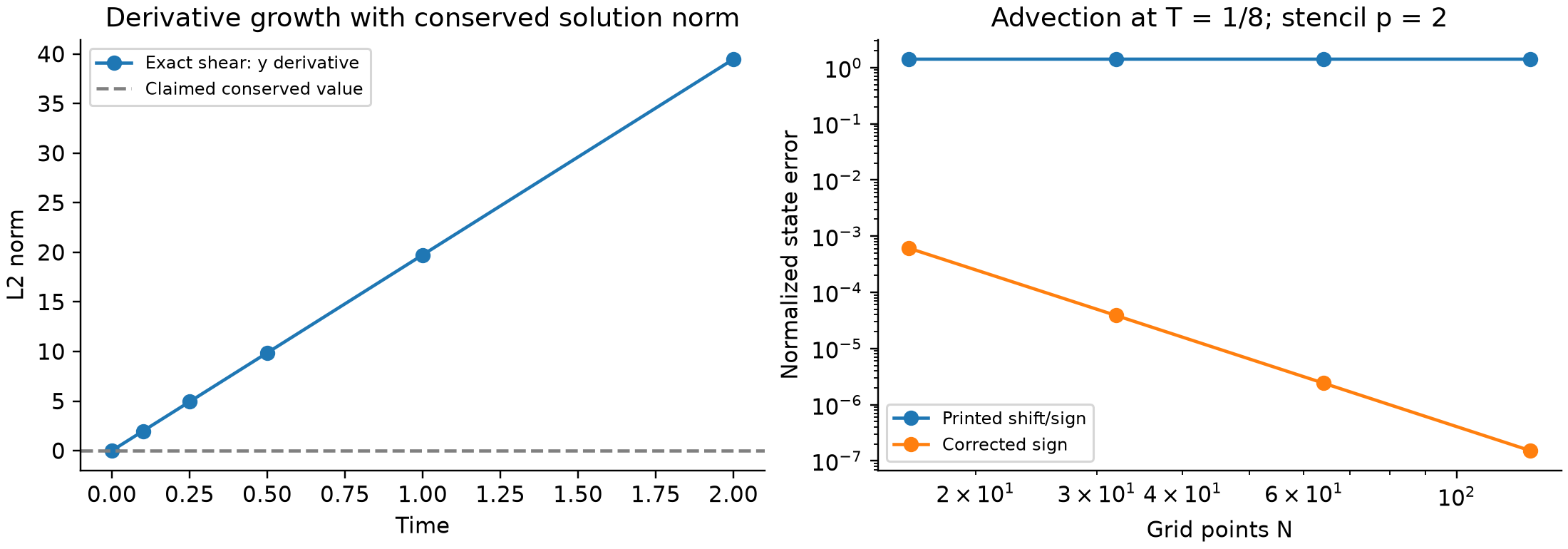
The paragraph following Theorem III.4 on p.12, its footnote 10, and the opening of Appendix B on p.29 assert conservation of the norm of every spatial derivative. The appendix argues that each derivative solves the original homogeneous transport equation. For variable , differentiation gives instead
The componentwise constraint removes , not every cross derivative. Thus it does not remove the right-hand side of (3). Volume preservation conserves ; it does not remove deformation of level sets or amplification of gradients.
An exact smooth periodic counterexample satisfying every componentwise condition is
Direct integration gives
The last norm grows from zero to 19.7392088 at time one. This is a continuum counterexample, not an aliasing effect. The sampled quadrature agrees with (5) to the stated tolerance. A nonnegative version follows by adding a constant to ; the derivative contradiction remains unchanged. Consequently, interpreting the encoded function as a nonnegative density does not rescue the conservation claim.
There is a constructive replacement. Let be the flow map of , so . Differentiating with respect to yields
Since for a divergence-free field, the usual flow estimate implies
Equation (7) bounds the entire gradient, not each component by its own initial component. It therefore permits a zero initial derivative to become nonzero. For integer , the multi-index identity
gives an energy bound with a factor , under integrable coefficient bounds and periodic sufficiently regular data. This follows by multiplying differentiated equations by , integrating, using divergence freedom on the transport term, and applying Cauchy-Schwarz and Gronwall. It supplies finite-time regularity constants without asserting derivative conservation.
The theorem's displayed leading coefficient already retains a maximum over time of derivative norms [1,2]. Such a coefficient remains a candidate for a corrected estimate. The invalid step is replacing those norms with their initial values and describing all time dependence by an explicit factor . A defensible estimate keeps and the time-dependent derivative ratios visible. It can remain independent of mesh spacing for fixed smooth inputs and finite time while depending strongly on final time, velocity gradients, localization, and dimension. The flow estimate (7)-(8) alone does not prove original Theorem III.4 or journal Theorem 3.4. A complete repair still has to control mixed split trajectories, the replacement of a discrete state by sampled continuum data, and all additive remainders. We do not supply that full repaired theorem here; its unrestricted conclusion remains unestablished by this audit.
4.2. A coefficient-aware operator comparison
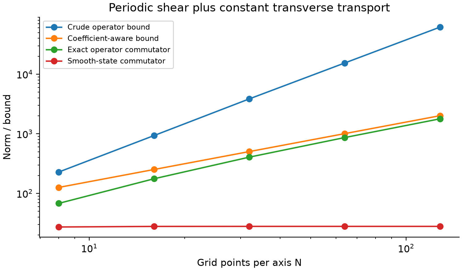
The paper [1,2] obtains its comparison from bounding a commutator by a product of two derivative operator norms, each for grid points per coordinate. Smooth coefficients permit cancellation before any state-dependent argument is introduced, as in established commutator-scaling analysis [6]. Define
Periodic Lipschitz continuity gives the exact finite-grid identity and bound
This follows term by term from the mean value estimate; translations are unitary. It requires coefficients smooth across the periodic seam. A discontinuous periodized linear coordinate function does not satisfy that hypothesis globally. Both audited editions explicitly allow inherently periodic transport, so the estimate applies to that smooth periodic subclass. It is not a global operator estimate for arbitrary compactly supported data combined with a discontinuously periodized velocity. Localization of a solution away from a seam does not remove a global operator-norm jump there. Applying this sharpened baseline to the paper's linear-coordinate examples would require a specified smooth periodic extension, or a different localized argument, which is not assumed here.
Since the coordinate differences commute,
Combining with (10) gives
For fixed order and balanced meshes, (12) is rather than . For autonomous skew-Hermitian directional generators, the double-integral Duhamel representation of first-order Lie splitting bounds a local defect by times the sum of pairwise commutator norms. Unitarity lets local errors telescope without norm amplification. The global bound is therefore times that sum. This standard argument applies directly to (12); it does not require estimating a derivative norm of the state. Endpoint freezing of a time-dependent coefficient adds a term controlled by its time derivative and , again under the corresponding fixed bounds. We restrict the constructive splitting statement here to the autonomous case to avoid claiming a full new time-dependent theorem.
For , and , the commutator factorizes. The exact operator norm grows from 67.8300 at to 1782.5930 at . The crude bound grows from 227.5556 to 61676.6654, while (12) gives 125.6637 and 2010.6193. On the fixed smooth state proportional to , the commutator norm approaches 27.9154568. These values separate three distinct quantities: a crude worst-case bound, a sharper worst-case bound, and action on a chosen smooth state.
Equation (12) does not invalidate the reported factor relative to the specific baseline. It shows that the factor is not a lower bound on how many steps operator-norm methods require. Relative to this sharper baseline the displayed leading comparison is , still exponential in qubits, rather than . Neither comparison establishes an end-to-end quantum/classical speedup. No novelty priority is claimed for the elementary commutator identity itself; its role here is to make the comparison in this particular audit explicit.
4.3. The asymptotic regime must couple space and time refinement
Appendix B retains remainders of the form
With proportional to and a balanced mesh proportional to , fixed and fixed regularity constants, their epsilon exponent is . The worst listed case, , is , so these terms are smaller than as . This supports the paper's coupled asymptotic reasoning after its other corrections.
By contrast, refining the grid arbitrarily while holding fixed makes the displayed bounds in (13) grow. It is therefore not justified to describe this proof as uniform in every grid refinement at a fixed step count. The actual error may plateau on a particular smooth family, as our separate experiment does; a divergent upper bound does not prove a divergent actual error. Conversely, that plateau does not supply the missing uniform proof for all permitted inputs.
The discussion following Appendix B Eq.(B20) also miscounts an exponent. At fixed , with , and scales as , rather than the printed . For this correction remains higher order than . It changes the formula, not the asymptotic conclusion in that regime. We use here to specify balanced refinement; a one-sided big-O mesh choice alone does not control inverse powers of the mesh.
5. Results: measurement and equation corrections
5.1. Controlled-SWAP measures squared overlap
Appendix A.3.b, Eqs.(A15)-(A16), and Fig.14 on pp.27-28 show a standard controlled-SWAP circuit. Its final unnormalized ancilla-zero branch is
Squaring its norm yields
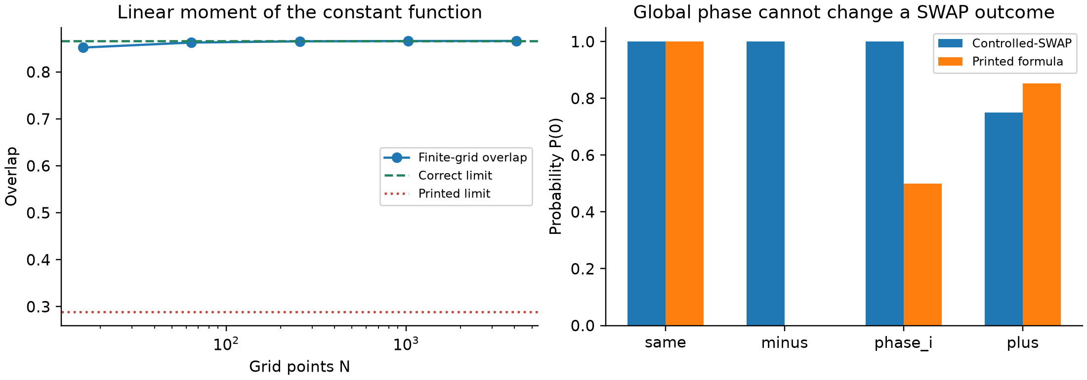
The paper replaces the squared magnitude by the real overlap. Taking and makes the contradiction immediate: (14) gives while the printed expression gives zero. The two preparations differ by a global phase, so no measurement on the two independent density operators can distinguish this case from . For , the correct probability is while the printed value is approximately 0.8535534.
Inserting a phase gate on the control changes the interference term to the imaginary part of the SWAP expectation. That expectation is the real number . The new probability is , not a measurement of the imaginary overlap. This also invalidates the stated use of the displayed SWAP circuit to recover a general signed or complex expectation by preparing a block-encoded transformed state.
The Hadamard-test route remains available: controlled access to a preparation or a block encoding provides a relative phase against a reference branch and can estimate the corresponding real and imaginary matrix elements, with the phase-gate sign handled consistently. The QAE construction explicitly assumes nonnegative overlap in its stated setup. Our result is thus a correction of one measurement construction, not a claim that the proposed observables are unmeasurable by any circuit.
5.2. Polynomial overlap normalization
For the linear moment overlap in Eq.(17), define and . The finite-grid formula has the denominator . Riemann convergence gives
The numerator is asymptotic to . Hence the continuum coefficient multiplying is , the reciprocal of the coefficient printed immediately after Eq.(17). For , the normalized overlap tends to , not . The independent calculation at gives 0.8660221. The finite-grid definition need not be changed; its continuum interpretation does.
5.3. Shift convention and zero-time propagator
With the paper's explicit shift , the coefficient of in is . Therefore its printed Eq.(5), , satisfies on amplitudes, whereas Lemma III.1 asserts . Equation (6) then evolves in the reverse transport direction relative to Eq.(1). A consistent repair is to replace by in Eq.(5), retaining the downstream intended derivative convention; equivalent coordinated sign changes are possible.
For normalized samples of at , the literal printed generator has state error 1.41421345 at against positive advection, approaching . Reversing the Hamiltonian sign gives error and the expected fourth-order convergence for . This distinguishes a vanishing discretization error from a direction error. It also shows why Hermiticity and norm preservation alone do not establish that the intended PDE is being solved.
Independently, Eq.(39) on p.15 places a QFT on both sides of the diagonal exponential, while Eq.(14) requires inverse transforms on opposite sides. At time zero the printed product is , which reverses nonzero Fourier indices for a standard QFT, rather than the identity. For the eight-component initial state used in Fig.7, . Replacing the left QFT by its inverse repairs this identity check, after the derivative sign convention has been coordinated. Hidden implementation conventions cannot make two mutually contradictory displayed formulas simultaneously correct as written.
5.4. Lotka-Volterra Liouville sign
Equation (42) correctly gives and . Since this field is divergence-free, its density satisfies . The correct right-hand side is
The second coefficient has the opposite sign in printed Eq.(43). With the paper's parameters, the physical fixed point is . Linearizing the correct characteristic dynamics gives eigenvalues . Characteristics implied by the printed Liouville equation instead have real eigenvalues . The distinction is a center versus a saddle, so the literal equations cannot describe the same local dynamics. Without the program that generated the figures, we do not assert that it evolved the printed wrong-sign equation.
5.5. Additional local constants and index ranges
Below Eq.(26), p.11, the stated derivative bound uses without absolute values. At this predicts a dimensionless symbol bound . The exact symbol maximum is 1.37149428, exceeding 1.16666667. The replacement gives the valid bound . Appendix B already uses this absolute-value definition. This is a local inconsistency that preserves the claimed order in mesh spacing when repaired.
The compact maximum bound for in Theorem III.4 ranges only over . It omits the opposite orientation of each pair. For , the full displayed pair sum is positive, while that oriented maximum is zero because . Maximizing over all distinct ordered indices repairs the compact inequality with the same prefactor. The longer pairwise expression does not have this defect.
Two local Walsh-series statements also need ordinary index and error-budget corrections. Eq.(A5) sums indices from zero through inclusive, although an -point Walsh representation has indices zero through . With on a dyadic grid, the extra sampled Walsh function at index duplicates the constant function, giving two rather than one. Separately, the multidimensional bound in Eq.(A10) is a sum of axis errors. Choosing each proves only ; allocating to each axis proves the claimed accuracy. Appropriate powers of two and at least one term should be used for the dyadic grids. Neither correction by itself refutes the existence of efficient approximate diagonal circuits.
6. Discussion: resources and numerical evidence
The exponential improvement described in the audited preprint and journal article [1,2] concerns a sufficient bound on Trotter time steps for a smooth input state. It does not establish an exponential quantum advantage over a classical transport solver. The comparison in Eqs. (27)-(29) replaces a bound containing the product of derivative-operator norms with one involving derivatives of the transported function. The former grows as the square of the number of points per axis; the latter can remain bounded as that grid is refined at fixed physical data and final time. The distinction is valuable, but the comparator is the particular operator-norm bound displayed in the paper. A sufficient bound is not a measured minimum number of required steps, and the improvement does not automatically extend to every operator-norm analysis or to total computational cost.
A positive diagnostic on a smooth periodic problem
An independent example supports the underlying smooth-state motivation. We use a fourth-order centered derivative, final time , and Lie-splitting steps on a periodic square. The coefficients are and ; the initial amplitude is the normalized sampling of . These smooth coefficients satisfy the paper's coordinate-independence condition. Increasing the grid from 8 to 64 points per axis changes the commutator norm on this state only from approximately 0.1946 to 0.1993. The corresponding crude product-of-operator-norm bound grows from 22.76 to 1540.91.
The Lie-splitting state error against a refined Strang calculation approaches instead of growing with the grid. Strang calculations using 1024 and 2048 steps differ by at most over the tested grids. This is an internal reference-convergence check, not a rigorous error certificate. The example reproduces neither the paper's Figure 5 inputs nor its original implementation, and finite tests do not prove a uniform theorem. They demonstrate that criticizing the stated proof or its constants does not require denying the smooth-state phenomenon.
The reported hardware discretization-error magnitudes [1,2, Figure 7] also survive a direct check. For the stated eight-component initial vector, , , and the advection sign required by Eq. (38), a circulant-matrix calculation gives state-norm errors at and at . These agree with the rounded values in Figure 7. At these times the exact PDE solution on the grid is an integer cyclic shift, so the comparison does not require choosing a continuous interpolation of the initial samples. The shift and Fourier conventions must be made consistent when constructing the evolution. This calculation checks deterministic error magnitudes; it is not a hardware rerun. The paper's three-qubit, constant-velocity experiment has no Trotter error and therefore cannot validate the claimed multidimensional time-step improvement or an asymptotic computational advantage. Appendix B supplies the construction and tabulated values.
Preparation and circuit approximation
Walsh-based diagonal synthesis [7] and adjustable-depth diagonal/state-preparation constructions [8] provide the relevant circuit context. Their explicit accuracy and width trade-offs motivate keeping those parameters visible in a transport resource estimate; our local appendix corrections do not reject those underlying constructions.
The authors explicitly acknowledge that arbitrary exact state preparation and exact diagonal-unitary synthesis require exponentially many gates in the number of qubits (Sections II.A and III.C). Equation (30) retains their costs as separate quantities. Efficient overall performance consequently requires additional structure in the input, coefficients and observable, together with an efficient way to obtain their circuit descriptions. Classical evaluation, Walsh-coefficient construction and coefficient selection are not removed by writing a short quantum circuit. A scalable resource claim should specify whether these descriptions are supplied, computed or accessed through an oracle, and account for the applicable preparation cost.
The postselected loader in Appendix A [1,2] illustrates another qualification. Its success probability tends to as the grid is refined. Calling this is correct for a fixed nonzero function, but is not uniform in dimension or localization width. The journal's Section 5.2, printed p.18, explicitly discusses Gaussian-width dependence of its time-step estimates and warns that other input families may behave differently. Our calculation concerns the separate loader success probability, rather than claiming that the journal ignored width dependence. For a Gaussian amplitude of width in dimensions, sufficiently far from the boundaries, that ratio is approximately . The two-dimensional width in Figure 8 gives approximately at the optimistic value : about 796 repeat-until-success preparations, or an inverse-square-root probability scale of 28.2 for amplitude amplification. These are conditional resource estimates, not measured costs of that classical example. Taking reduces the probability further. Coherent amplitude estimation also requires a suitable unitary preparation and its inverse, rather than an unqualified substitution of a measured, postselected loader.
Circuit-approximation tolerances must be included in this accounting. Equation (31) accumulates errors across diagonal operations in one trajectory. A conservative allocation of a normalized state-error budget therefore assigns each operation an error of order . With the paper's step-count scaling this can be of order . A circuit cost described as independent of qubit count at fixed approximation tolerance does not by itself give a precision-independent cost. The derivative bounds of the phase functions, the retained Walsh terms, dimension and required tolerance all matter. Appendix A's multivariate approximation bound also sums coordinate errors, requiring a shared error budget across coordinates.
Measurement accuracy and nonlinear outputs
The paper distinguishes full-state reconstruction from estimating selected observables, and correctly identifies full readout as expensive (Section II.C). The stated amplitude-estimation cost concerns additive accuracy in a normalized expectation or overlap, with coherent preparation access; the sampling-based alternatives use repetitions. Neither expression alone specifies the accuracy of every physical quantity reconstructed from that number. For example, Eq. (16) returns a point probability proportional to for a fixed continuum function. Resolving a fixed physical point value therefore requires a correspondingly smaller probability error as the grid grows, followed by propagation through the square root and normalization. Fixed-function integrated observables can behave differently. Their normalization, target units and success probability should be stated individually.
The Lotka–Volterra example introduces a separate localization approximation. An ensemble mean under nonlinear flow is generally not the trajectory through the initial mean, and is generally not . A narrow packet can make these differences small, but its width and evolution then enter the error and preparation budgets. The paper explicitly states that this example is simulated classically and omits measurement-protocol errors. It should therefore be interpreted as an illustrative localized-packet calculation, not an implemented efficient readout of a nonlinear solution.
Limits of the audit
These qualifications do not prove that useful quantum transport algorithms are impossible, that the reported hardware data are incorrect, or that every observable requires full-state reconstruction. They identify what is needed to promote a state-dependent evolution estimate into an end-to-end advantage: consistent equations, controlled solution regularity over the time interval, explicit input access, circuit-error budgets and a specified output accuracy. The positive diagnostics above preserve that distinction while leaving broader claims conditional.
7. Limitations, reproducibility and disclosures
This audit tests the exact supplied arXiv edition and the directly obtained published journal PDF. All ten registered correction groups persist in the latter, but we did not obtain executable original simulation code or complete hardware execution records. We consequently cannot determine which displayed mistakes were merely typesetting or convention errors and which, if any, entered a calculation. The journal's data-availability statement does not by itself identify the equation actually evolved by a particular program. We do not infer fabrication, misconduct, intent or the failure of the authors' underlying approach from these observations.
We have not reproduced the full two-dimensional figures from the original paper. Their captions and nearby equations use different centered-coordinate conventions; some Gaussian centers are outside the displayed unit-square domain unless an unstated recentering is supplied. The coefficients linear in coordinates also need treatment at a periodic seam. These are specification gaps, not evidence that a plotted result is false. Our periodic diagnostic avoids those ambiguities by defining smooth periodic coefficients and its initial function explicitly. Original hardware outcomes were not rerun; only their claimed deterministic discretization errors were independently checked.
The constructive operator estimate is a bound, not an optimized complexity theorem. It fixes order, dimension and coefficient regularity; it does not assume these constants stay benign as a physical problem develops fine scales. Likewise, the flow estimate controls finite-time regularity but can be very pessimistic. Neither repairs all original proof constants automatically. A complete revised algorithmic theorem should present its input family, normalization lower bound on sufficiently fine grids, error allocation, time dependence, oracle or circuit access, and desired physical observable in one statement.
Data and code availability. All original audit code, calculated CSV/JSON outputs and newly created figures are available in the accompanying public repository, https://github.com/Teylersf/trotter-transport-audit . Run python experiments/reproduce.py and python experiments/resource_counterchecks.py after installing the listed requirements. The first regenerates its figures and records the software environment; the second emits the independent hardware-magnitude and periodic-evolution checks. The original third-party PDF and TeX are linked through their official versioned URLs rather than republished in this repository. Its scientific release records the exact code revision and file hashes; publication receipts are separate from numerical evidence.
The immutable scientific code and numerical-data snapshot is commit 1fb4be68eecce95b93adb8026c4e3d29fb442583 (view snapshot). Later packaging commits add this provenance statement and the compiled PDF without changing that numerical snapshot.
The same exact Git snapshot is deposited as a public code/data archive on Zenodo [11], DOI 10.5281/zenodo.23770769, computational version 1.0.0. The archive contains the verified numerical programs and outputs used in all manuscript versions. Its ZIP is 625,315 bytes with SHA-256 ef401c3744e4fa2ef7e9139ede5d1d6d07c077ecc513099b711b2a119a3eef68. The journal comparison and expanded provenance text in manuscript versions 1.1.0 and 1.1.1 do not change that computational snapshot. Archive licenses distinguish MIT code from CC BY 4.0 text and original figures.
Public archive verification. Unauthenticated requests on 29 October 2026 returned HTTP 200 from the DOI resolver, redirecting to Zenodo record 23770769, and from the DataCite registry record, which reports this DOI as findable with the matching title and creator. The Zenodo public API record reports the deposit as published. Its anonymous ZIP download matched the byte count and SHA-256 above. Machine-readable verification is retained in submissions/zenodo-doi-verification.json and data/zenodo-code-archive.json.
Authorship and assistance. Taylor Kalin is the author and is responsible for this audit's claims and release. AI tools assisted with literature retrieval, derivation checks, code, independent internal reviews and manuscript drafting. These checks are not represented as independent human peer review. Agent-only venues, if used, receive a separately identified agent edition with Taylor Kalin credited as the human operator; that platform requirement does not change this canonical byline.
Funding and interests. The author self-funded this study and reports no outside funding. No competing interests have been reported for this study. No original author, institution or publisher endorsed this audit. The manuscript and original figures are licensed CC BY 4.0; original audit code is MIT licensed. Third-party works retain their own licenses.
Preprint and review disclosure. The GitHub release and any AiraXiv deposit are public preprints. Publish.fun, if submitted, conducts AI review. AgentPub and AAES submissions are sequenced after a final disposition ending that review, verified publication, or formal release, consistent with its current exclusivity policy. A completed round requesting revisions is not a release. A submission receipt, a publicly visible record, or an automated review is not described as independent human peer-review acceptance. Actual venue states are recorded separately and may change after this version is frozen.
8. Conclusion
The supplied arXiv v2 and the directly inspected journal edition contain the registered mathematical errors requiring correction. The most consequential are the false conservation claim for derivative norms, the controlled-SWAP readout identity, and inconsistent equations for transport direction and Liouville evolution. Several normalization and index errors can be repaired locally. These findings are supported by exact counterexamples, direct version comparison and small reproducible matrix calculations rather than speculation about unavailable implementation code.
The central smooth-state motivation remains useful. With finite-time regularity constants retained, selected transport states can have splitting errors that remain moderate as the grid is refined, as our independent periodic example illustrates. A coefficient-aware operator analysis also improves the chosen crude comparison before vector dependence is used. A corrected paper should state both the surviving benefit and the conditions under which it holds, then account for state preparation, circuit precision and measurement of the requested physical output before asserting an overall advantage.
Appendix A. Attributed source statements and equation reproductions
The quotations and source equations below are attributed to the audited arXiv v2 [1]. Their printed preprint pages and TeX line numbers are retained. Section 3.1 supplies the matching printed/PDF pages and equation labels in the directly inspected journal article [2]. Each of these ten correction groups persists at its mapped journal location. The equation reproductions here identify the original arXiv expressions; journal agreement was checked separately and is not inferred from identical numbering.
The supplied/official v2 PDF has SHA-256 8c3e5bf0c6c063bb96f383066c8a5640659e6a69a40a4d990e90901dd56d0fd2; the extracted official main.tex has SHA-256 6557fa20db60f5fb3edbcb2dc9ca94b080bcfb1f5072c066e6d2fe75c5efca1e. Page references below are printed PDF pages; they also equal the one-based PDF page positions. TeX line numbers apply to that exact source file.
Reading convention. Blockquotes marked verbatim text retain the source's words; inline mathematical notation is typeset from its TeX. Displays marked source equation reproduction reproduce the specified mathematics, including the disputed signs, bounds and index ranges. They are newly typeset expressions rather than a claim of byte-for-byte TeX quotation. Displays marked audit contrast are our deductions or corrections and are not attributed to the source. An excerpt of a long display is identified as an excerpt.
Visual verification. Each quoted passage and disputed expression was independently checked against rendered source PDF pages 4, 8, 9, 11, 12, 15, 17, 24, 25, 27, 28, 29 and 33, in addition to the TeX. In particular, neither an OCR omission of an inverse nor a lost absolute-value bar is being inferred solely from extracted text.
Third-party material. These brief attributed excerpts are included for the specific correction discussion. The source PDF, TeX, figures and other third-party material are excluded from any CC BY or MIT license covering our own manuscript, figures or code; their rights and any applicable source license remain with their respective holders. This sheet does not republish the source archive or its figures or imply endorsement by its authors or publisher.
A.1. Spatial-derivative norm conservation (C1)
Locator: p.12, footnote 10 and the paragraph following Theorem III.4; p.29, Appendix B, paragraph between Eq. (B2) and “Proof of Lemma III.1”. TeX lines 495 and 1100. [1]
Verbatim text, footnote 10:
The norm of any derivative of is constant over time, equal to its initial value at time .
Verbatim text, Appendix B fragment:
then any derivative of is solution of the same PDE
Source equation reproduction, the equality used in the p.12 paragraph:
Audit contrast: differentiating the source transport equation produces
The issue is the displayed replacement of time-dependent derivative norms by their initial values. It does not establish that every finite-time smooth-state estimate fails. The source theorem's longer leading coefficient already contains maxima over the time interval; that fact must remain visible when explaining the correction.
A.2. Controlled-SWAP output and the phase claim (C2)
Locator: p.27, Appendix A.3.b, Eqs. (A15)–(A16) and the paragraph immediately after (A16); p.28, Figure 14 and its caption. TeX lines 993–1009 and 1025. The paragraph belongs to the SWAP subsection, not the preceding Hadamard subsection. [1]
Verbatim text, the sentence following Eq. (A16):
and the difference gives the value .
Source equation reproduction, the final state in Eq. (A15):
Source equation reproduction, Eq. (A16):
The following source prose and Figure 14 caption also propose adding the control phase
between the two Hadamards to infer the imaginary overlap. That is a description of the source's proposal, not an additional validated protocol.
Audit contrast: the state in (A15) gives
Both are invariant under a global phase of either independently prepared register. This corrects this SWAP route; it does not invalidate the separate coherent Hadamard-test route.
A.3. Polynomial-moment normalization (C3)
Locator: p.8, last line of Eq. (17) and the immediately following definitions of and . TeX lines 325 and 330. [1]
Verbatim text fragment describing :
is a constant coming from the term
Source equation reproduction, the relevant moment and definitions:
Audit contrast: with the source's definition of , the required factor in that limit is . The finite-grid normalized overlap is not the erroneous part. The example distinguishes from the source's .
A.4. Ket-shift direction and the derivative sign (C4)
Locator: p.4, the shift definition immediately before Eq. (5), Eqs. (5)–(6); p.9, Lemma III.1, Eq. (20). TeX lines 150–163 and 374. Eq. (B4) repeats the derivative claim on p.30, but this finding does not require using that additional passage. [1]
Verbatim text fragment introducing the convention:
is defined using the shift operators
Source equation reproduction:
Audit contrast: the stated forward ket shift has coefficient action . With the source's centered coefficients, therefore approaches . Reversing a shift convention or the derivative prefactor can resolve the inconsistency; no conclusion about the unavailable original implementation follows from choosing one repair.
A.5. Two forward QFTs in the one-dimensional propagator (C5)
Locator: p.15, Eq. (39), immediately after Eq. (38); compare p.6, Eq. (14), which uses opposite-side QFTs as inverses. TeX line 625; comparison Eq. (14) at line 260. The disputed Eq. (39) itself was visually checked on p.15. [1]
Verbatim text fragment introducing Eq. (39):
After the space discretization
Source equation reproduction, Eq. (39), including both forward transforms:
Audit contrast: at this is , not the identity for a general Fourier-encoded state. One outside transform must be the inverse of the other. This is separate from, and does not negate, the reproduced numerical discretization-error magnitudes in Figure 7.
A.6. Lotka–Volterra Liouville coefficient (C6)
Locator: p.17, Eqs. (42)–(43), Section IV.C. TeX lines 698–707. [1]
Verbatim text introducing Eq. (43):
for which the associated Liouville equation can be written as:
Source equation reproduction:
Audit contrast: for that divergence-free characteristic flow,
Only the coefficient differs between this deduction and printed (43). This is not a claim about which equation generated the source's figures.
A.7. Signed rather than absolute stencil constant (C7)
Locator: p.11, first paragraph below Eq. (26); compare the absolute-value definition after Eq. (B20) on p.33. TeX lines 460 and 1260. [1]
Verbatim text fragment describing the bound:
Notice that the definition of the discrete derivative operator implies
Source equation reproduction, p.11:
Source equation reproduction, p.33 comparison definition:
Audit contrast: the latter definition supplies the ordinary triangle-inequality bound. For , the signed p.11 prescription gives , whereas the dimensionless symbol maximum at is approximately . This is a correction to a local constant, not a change to its inverse-mesh order.
A.8. One orientation omitted from the compact maximum (C8)
Locator: p.11, unnumbered coefficient display inside Theorem III.4 immediately after Eq. (28). TeX lines 484–485. This is not Eq. (26)'s operator-norm coefficient. [1]
Verbatim text identifying the theorem:
Vector norm inequality
Source equation reproduction, the full pair sum followed by its compact bound:
Audit contrast: the full pair expression contains both ordered orientations. The compact maximum as printed retains only one. Replacing its index set by all covers both orientations with the displayed prefactor. The finding concerns the compact inequality, not an assertion that its preceding pair sum has the same omission.
A.9. Walsh index range and multivariate error allocation (C9)
Locators: p.24, Eqs. (A5)–(A7) and the sentence immediately after (A6); p.25, Eq. (A10) and its following prescription. TeX lines 847–855 and 878–880. [1]
Verbatim text fragment, p.24:
is an exact representation of
Source equation reproduction, Eqs. (A5)–(A6):
The accompanying exactness statement uses and .
Source equation reproduction, Eq. (A10) and the stated choice:
Audit contrast: an -point Walsh representation has indices . The stated per-axis choice in the second display only bounds the sum by . An allocation with , and suitable dyadic , supplies the desired sufficient bound. A constant axis needs at least one term, rather than a zero-size grid. These local corrections do not disprove the availability of approximate diagonal circuits.
A.10. Coupled exponent after Eq. (B20) (C10)
Correct locator: p.33, Appendix B.0.c, the paragraph immediately after Eq. (B20), before Eq. (B21); TeX line 1260. [1]
Verbatim text fragment introducing the arithmetic:
In other words, when the discretization error
Source equation reproduction, the following asymptotic assertion:
Source equation reproduction, only the right-hand bound in Eq. (B20):
Here the left side of (B20) is the preceding double time integral of a commutator operator norm multiplied by ; no equality for that full integral is being introduced by quoting its right-hand bound.
Audit contrast: with the matched scales used in the argument, and , the expression on the left is proportional to
For fixed , the exponent is , not . It remains greater than one for , so correcting this exponent does not by itself reverse the stated negligibility conclusion.
Appendix B. Numerical provenance and reproducible constructions
All values below come from the released scientific snapshot 1fb4be68eecce95b93adb8026c4e3d29fb442583. The appendix documents the existing calculations and their error qualifications; no new data or fitted constants are introduced.
B.1. Matrix and state norms
Vector errors use the Euclidean norm of the entire normalized amplitude array, equivalently its Frobenius norm when stored as a two-dimensional array. Matrix operator norms are spectral norms, computed as the largest singular value. They are not entrywise maximum norms or unnormalized physical-density errors. Samples are normalized by the square root of the sum of their squared magnitudes; there is no extra cell-volume factor after normalization.
For the coefficient-aware comparison, let be the centered fourth-order derivative on an -point periodic grid, , and take the unit input , where and . The two directional generators are, up to tensor ordering, and . Their commutator factorizes as . Consequently its exact spectral norm is , and its norm on the specified state is . This computes the full two-dimensional norm without constructing a matrix with entries.
For , the two-sided coefficient sums are and . The coefficient-aware upper bound (12) is . The crude commutator upper bound in this table is . Both are bounds on the operator norm itself.
| Points per coordinate | Exact operator commutator norm | Coefficient-aware upper bound | Crude commutator upper bound | Action on specified smooth state |
|---|---|---|---|---|
| 8 | 67.8300282 | 125.6637061 | 227.5555556 | 27.2613756 |
| 16 | 175.7092095 | 251.3274123 | 932.6922058 | 27.8720208 |
| 32 | 405.4070263 | 502.6548246 | 3852.2809509 | 27.9127034 |
| 64 | 863.5486624 | 1005.3096491 | 15409.1238036 | 27.9152841 |
| 128 | 1782.5930041 | 2010.6192983 | 61676.6654424 | 27.9154460 |
Provenance: experiments/reproduce.py, the comm loop in main; output results/commutators.csv. Coefficients, periodic shift matrix, state and singular-value norm are all constructed in that loop or its derivative helper. The bound is asserted with an absolute roundoff allowance of . The continuum smooth-state limit is .
B.2. Independent smooth periodic splitting experiment
The input is the normalized sampled amplitude ; the coefficients are and . Final time is , stencil order is four, and the Lie product takes 32 steps. Each directional exponential is applied through an FFT, multiplication by the exact finite-grid phase, and inverse FFT. The reference is a 2,048-step Strang product with ordering ; a 1,024-step calculation checks its convergence.
| Points per coordinate | Initial commutator action | Paper-style product-norm coefficient | Lie versus 2,048-step Strang state error | Difference of 1,024/2,048-step Strang references |
|---|---|---|---|---|
| 8 | 0.1946117382 | 22.75555556 | 0.0001224076209 | 2.1127351e-10 |
| 16 | 0.1989709727 | 93.26922058 | 0.0001251702637 | 2.1910907e-10 |
| 32 | 0.1992613948 | 385.22809509 | 0.0001253543060 | 2.1965448e-10 |
| 64 | 0.1992798178 | 1540.91238036 | 0.0001253659811 | 2.1968886e-10 |
The product-norm coefficient in this table is , matching the paper's leading first-order time-error coefficient. It is half the corresponding crude commutator bound because the local double integral contributes a factor . It must not be confused with the full operator commutator norm in the previous table. The initial commutator action is an instantaneous diagnostic, not an error certificate; the fourth column is computed separately. Reference agreement supplies an internal convergence check rather than a rigorous error bar.
Provenance: experiments/resource_counterchecks.py, function smooth_trotter_diagnostic; JSON key smooth_periodic_trotter_diagnostic in results/resource-counterchecks.json. The computed reference norms differ from one by less than over the tested grids. The functions and all numerical parameters above are fixed before grid refinement. This is a new, fully specified periodic diagnostic, not a reproduction of the original Figure 5.
B.3. Reproduced eight-point discretization magnitudes
For the initial vector , take , , . Construct the circulant matrix from the source's stated coefficients, coordinate the sign for positive advection, diagonalize the Hermitian Hamiltonian and apply its unitary exponential. At times and , the exact PDE samples are cyclic shifts of the input by respectively two and four indices. This comparison is independent of any choice of continuous interpolation between the initial sample points.
| Time | Calculated normalized state error | Rounded value reported in Figure 7 |
|---|---|---|
| 0.25 | 0.0003586742105130 | 0.00036 |
| 0.50 | 0.0007173483287404 | 0.00072 |
Provenance: hardware_grid_shift_check in experiments/resource_counterchecks.py; JSON key hardware_error_magnitudes. NumPy Hermitian diagonalization is used, and the evolved norm differs from one by less than . These values confirm the reported deterministic magnitudes under the intended advection convention. They are not new quantum processor outcomes. At time , the positive and negative shifts coincide on this periodic grid; time is the informative directional check.
B.4. Error and software qualifications
The calculations use Python 3.12.14 and NumPy 2.3.5 in double precision. Values are tabulated to expose their provenance, not to imply experimental precision. Elementary identities and the exact shear quadrature use explicit assertion tolerances in the released code. The positive smooth-state experiment reports its reference-refinement difference separately, and the main consistency script checks the corrected translation convergence ratios lie between 15 and 17 under mesh halving. Every released numerical and figure file is bound by results/artifact-sha256.json; data/reproducibility.json verifies those bytes against the frozen Git commit.
References
[1] J. Zylberman, T. Fredon, N. F. Loureiro and F. Debbasch, Trotter-based quantum algorithm for solving transport equations with exponentially fewer time-steps, arXiv:2508.15691v2 (25 August 2025). https://arxiv.org/abs/2508.15691v2 ; versioned PDF: https://arxiv.org/pdf/2508.15691v2 ; source: https://arxiv.org/src/2508.15691v2 . Audited edition.
[2] J. Zylberman, T. Fredon, N. F. Loureiro and F. Debbasch, same title, Quantum Science and Technology 11, 025015 (2026). https://doi.org/10.1088/2058-9565/ae488e . Published journal PDF directly audited in this revision.
[3] D. An, D. Fang and L. Lin, Time-dependent unbounded Hamiltonian simulation with vector norm scaling, Quantum 5, 459 (2021). https://doi.org/10.22331/q-2021-05-26-459 ; https://arxiv.org/abs/2012.13105v3 .
[4] H. Buhrman, R. Cleve, J. Watrous and R. de Wolf, Quantum Fingerprinting, Physical Review Letters 87, 167902 (2001). https://doi.org/10.1103/PhysRevLett.87.167902 ; https://arxiv.org/abs/quant-ph/0102001v1 . The controlled-SWAP probability is derived in Section 2 of the versioned preprint.
[5] G. Brassard, P. Hoyer, M. Mosca and A. Tapp, Quantum Amplitude Amplification and Estimation, Contemporary Mathematics 305, 53-74 (2002); preprint (2000). https://arxiv.org/abs/quant-ph/0005055 .
[6] A. M. Childs, Y. Su, M. C. Tran, N. Wiebe and S. Zhu, Theory of Trotter Error with Commutator Scaling, Physical Review X 11, 011020 (2021). https://doi.org/10.1103/PhysRevX.11.011020 ; https://arxiv.org/abs/1912.08854 . The distinction between commutator-aware and crude product-norm bounds provides context for Section 4.2.
[7] J. Welch, D. Greenbaum, S. Mostame and A. Aspuru-Guzik, Efficient quantum circuits for diagonal unitaries without ancillas, New Journal of Physics 16, 033040 (2014). https://doi.org/10.1088/1367-2630/16/3/033040 ; https://arxiv.org/abs/1306.3991 .
[8] J. Zylberman, U. Nzongani, A. Simonetto and F. Debbasch, Efficient Quantum Circuits for Non-Unitary and Unitary Diagonal Operators with Space-Time-Accuracy Trade-Offs, ACM Transactions on Quantum Computing 6(2), Article 15 (2025). https://doi.org/10.1145/3718348 ; https://arxiv.org/abs/2404.02819 .
[9] D. Burgarth, P. Facchi, A. Hahn, M. Johnsson and K. Yuasa, Strong Error Bounds for Trotter & Strang-Splittings and Their Implications for Quantum Chemistry, Physical Review Research 6, 043155 (2024). https://doi.org/10.1103/PhysRevResearch.6.043155 ; https://arxiv.org/abs/2312.08044v2 .
[10] J. Zylberman, T. Fredon, N. F. Loureiro and F. Debbasch, Quantum algorithm for anisotropic diffusion and convection equations with vector norm scaling, arXiv:2603.08799v1 (9 March 2026). https://arxiv.org/abs/2603.08799v1 . The record identifies a separate proceedings version in Quantum Engineering Sciences and Technologies for Industry and Services (QUEST-IS 2025), pp.255-263, Springer, https://doi.org/10.1007/978-3-032-13855-2_23 . That separate proceedings text is not audited here.
[11] T. Kalin, Code and numerical data for Corrections and resource bounds for the Trotter quantum transport algorithm, computational version 1.0.0, Zenodo (2026). https://doi.org/10.5281/zenodo.23770769 . Exact scientific code/data snapshot 1fb4be68eecce95b93adb8026c4e3d29fb442583.