Abstract
Regional particle energization requires tracking where each energy increment occurs. We audit the posted particle-attribution routine associated with arXiv:2511.15988v1 and analyze all 1,003 histories in its two publicly released example batches. The routine partitions trajectories at first sheet and subsequent downstream passages; later returns do not change that chronological attribution. A zero-transition-increment counterexample reverses regional ordering while preserving total-gain closure. Applying the routine to four released illustrations reproduces all eight preprint annotations, and three illustrations exactly match full histories in the larger batch. Pooling the batches before applying the source's strict final-energy cuts leaves 667 intermediate and 84 high-energy histories. In the available high-energy subset, the downstream particle-mean fraction changes from 0.500318 under first-passage attribution to 0.370129 under symmetric full-history attribution; left and right conventions give 0.370742 and 0.369515. Its fraction of total net gain changes from 0.490959 to 0.393724. Downstream remains dominant in the intermediate subset. All comparisons retain signed increments and identical particle selections. The batches have undocumented release probabilities and do not reproduce the published intermediate-band point; these are measured available-sample effects, not a corrected full-population result. Discrete endpoint allocations also do not uniquely recover continuous electric work. Supporting appendices preserve positive initialization and diagnostic-curve checks, distinguish inferred plotting operations from source-unit evidence, and print the complete audited routine.
Editorial notes
Points the editor recorded on accepting the paper. They are published with the article; the authors were not required to address them before publication.
- Section 5, 'Available cohort and paired analysis', still describes source-function agreement as checked on '32 histories per staging batch'; revise this sentence to point to the later complete-function validation on all 1,003 histories.
- Section 7 documents DataCite and doi.org resolution for [9] and [10] only; add the corresponding dated resolution check for the v1.2.0 archive [12].
- Abstract and Section 8: mention the conditional bootstrap range for the high-band shift alongside the 13.0189-point figure, with its stated non-population interpretation.
- Section 3, third paragraph: replace 'A subsequent revision additionally examines' with a direct statement of the analyzed batches, so the text does not read as a revision log.
First-passage attribution and regional particle energization in multiscale reconnection
Taylor Kalin
Independent researcher; https://taylorkalin.com
ORCID: 0009-0003-9000-9315; correspondence: teylersf@gmail.com
Version 1.2.0; 29 October 2026
1. Introduction
Magnetic reconnection transfers energy across kinetic and macroscopic scales. A simulation can show that energetic particles visit several regions, while answering several distinct questions about their histories: where they gain energy, how much they gain after leaving a particular site, and which forces or mechanisms supply that gain. These questions require different diagnostics. A chronology of first passages is useful for transit and injection studies. A spatial budget instead requires the region occupied during each contribution to the energy change.
Velberg and colleagues [1] study the coalescence of magnetic islands in a relativistic electron-positron plasma. Their fully kinetic calculations develop a primary reconnecting sheet, ejected plasmoids, secondary sheets and downstream activity. The paper reports electron-frame nonideal-work diagnostics partitioned across these regions, energy spectra, and gains along selected particle trajectories. It concludes that downstream activity becomes an important energy-conversion and particle-acceleration channel as the system grows. The present audit concerns how regional particle gains are calculated and interpreted, with separate checks of the initial field and the released diagnostic evidence.
The paper's region decomposition is dynamic. Four initial particle tags identify the two islands and the top and bottom populations. Their evolving mixture, together with a geometric current-sheet classifier, defines the regions used by the analysis. The original supplemental material describes a 99 percent island-density criterion, an effective sheet-width parameter related to island height, and an additional two-skin-depth expansion of the sheet mask. A trajectory can therefore change region as it moves and as the diagnostic boundaries evolve. Its tag at initialization and its region at a later time have different meanings.
For a particle with Lorentz factor , the laboratory kinetic-energy change is proportional to the integral of electric work. Its partition into regions depends on the region indicator at the time of that work. In the deposited implementation [2], however, the regional attribution is calculated from the Lorentz factors at first sheet entry, first subsequent downstream entry and the final sample. Such endpoint differences automatically close the total budget. They do not retain the locations of later returns. The distinction is directly testable without rerunning a large particle-in-cell simulation.
Our main result is a source-specific method discrepancy, supported at four levels. First, inspection of the pinned routine identifies its chronological partition. Second, controlled traces give exact counterexamples, including one inside the source's reported intermediate energy band, for which energy-changing intervals have fixed region labels and all transition increments vanish. Third, the four released illustrative trajectories reproduce the eight energy annotations printed in the preprint. Fourth, a paired reanalysis of every history in the two released batches measures the difference between first-passage and full-history discrete alternatives under both averaging conventions. Three illustrations exactly match full released-batch histories, strengthening that example-level provenance. The discrete alternatives remain sampling conventions, not uniquely established continuous-time energy budgets.
The contribution is deliberately bounded. We do not infer a population-wide correction from the released convenience batches or the four author-selected illustrations. The available intermediate-band first-passage mean does not reproduce the original Figure 6 point, which directly cautions against identifying the public union with the full historical cohort. Nor do we treat a discrepancy in a particle diagnostic as a disproof of the separately measured downstream nonideal-work activity. Appendices retain its positive curve reconstruction and the initialization checks. The main text leads with the paired empirical effect and separates that measured result from an unmeasured change to the complete published population.
2. Related work and diagnostic context
The source simulation uses VPIC, a general-purpose relativistic particle-in-cell code whose numerical framework and computational scale are described by Bird et al. [6]. This audit analyzes released diagnostics and small exact constructions. It neither reproduces the full simulation nor attributes the analysis-function discrepancy to the underlying VPIC particle pusher. The posted input decks and diagnostic scripts are distinct evidence artifacts and are treated separately.
Particle acceleration studies distinguish injection and later energization, as well as contributions associated with parallel electric fields, Fermi processes and pickup. French et al. [5], for example, investigate guide-field and system-size dependence using particle histories and field-based diagnostics. Those physical mechanisms cannot generally be identified from a region name alone. Conversely, the time at which a particle first reaches a region does not specify where all its subsequent work occurs. Our analysis addresses this latter aggregation issue; it does not introduce a new acceleration mechanism.
The electron-frame measure introduced by Zenitani et al. [3] is a Lorentz-invariant scalar for the selected electron-fluid reference. It is valuable for locating nonideal energy conversion. Distinctions among field work, bulk flow, internal energy and other dissipation surrogates are established topics, including the comparisons of Pezzi et al. [8] and Yang et al. [7]. We use those distinctions to delimit what is being checked. A cumulative region-resolved proxy, a laboratory electromagnetic-energy budget and a particle-selected gain statistic need not be the same observable.
The initial island field is described in [1] as a force-free modification of the Fadeev configuration [4]. Elementary divergence and curl identities provide a direct consistency check, independent of numerical evolution. They also make it possible to identify a printing discrepancy while confirming the currently posted input expression. We do not claim novelty for these field identities, for telescoping sums, or for the covariance identity relating two averaging conventions. The new application is the audited relationship among the specific deposited routine, the reported illustrative values and a time-local regional-work interpretation.
3. Source provenance and released particle data
The audit fixes its scientific target to the eleven-page arXiv:2511.15988v1 preprint by Velberg and collaborators. The supplied PDF is byte-identical to the official versioned download, with SHA-256 c2648dcac8e67dc1136dc4f6339166cb475ebe44a7415508a97e34f0056a5b48. The official record, checked on October 29, 2026, lists one version, submitted November 20, 2025. The PDF's November 21 typesetting date does not establish another scientific revision: its source uses a current-date typesetting command. We read the complete PDF and TeX, including the supplementary material. The bounded primary-metadata checks did not identify a journal article or erratum. This is an edition-specific audit, not a claim that no later publication can exist. Velberg et al., arXiv:2511.15988v1.
The associated OSF deposit materially improves what can be checked. Its exact title, Alexander Velberg's creator record, and author-naming project wiki establish the association. The deposit has a registered DOI, 10.17605/OSF.IO/EPWTU, and supplies example VPIC decks, custom diagnostic includes, postprocessing programs, processed arrays and selected particle histories. The project was created December 5, 2025; its current README is marked July 20, 2026. These dates postdate the audited preprint. The README also uses a later figure layout: its cumulative-proxy “Figure 4” data correspond to preprint Fig. 3, its instantaneous-proxy “Figure 3” data to preprint Fig. 4, and its particle-fraction “Figure 5 Bottom” topic to preprint Fig. 6. The additional global-energy and regional material is assigned other later figure numbers. This mapping is recorded explicitly; the deposit is not silently treated as a hash-identified snapshot of every program that produced v1. Velberg, OSF EPWTU.
The frozen inventory contains 182 files. To bound transfer while examining the relevant methods, we retrieved and verified the 127 files no larger than two megabytes individually. These include the input decks and postprocessing needed here. A subsequent revision additionally examines the complete publicly posted intermediate-energy p008 and high-energy p000 batches, with their paired trajectory and region time chunks. These are documented example batches, not the entire simulation population or an established probability sample. The project describes its much larger underlying dataset and offers additional data on request. Consequently, the audit distinguishes a reproduced calculation on available files from a complete rerun of the approximately forty-billion-particle simulation. The numeric OSF fixtures are preserved under the project's CC0 license; that license does not replace independently applicable upstream software licenses. Coordinates derived from the preprint's figures are separately attributed under its CC BY 4.0 terms.
The manuscript distinguishes three provenance claims. The December 2025 routine is directly inspectable and explicitly identifies the relevant particle-energy figure in its comments. Its outputs on the four released illustrations reproduce the eight v1 annotations. Neither this agreement nor the later figure-generation comments establish a hash-identified November 2025 executable or the exact Figure 6 cohort. The new batch comparison holds each released history fixed while changing only the attribution ledger; it does not silently identify those batches with the complete v1 population.
The source and software DOIs are registered by DataCite. Public DataCite metadata, the doi.org registration-authority service and anonymous downloads were checked directly; absence from a Crossref lookup is not absence from the DOI system. Direct source access is https://osf.io/epwtu/ and the original software record is https://zenodo.org/records/23774456 . Public verification receipts preserve the registry URLs, metadata and downloaded-file checksums. The full pinned routine is printed in Appendix D. Positive field and proxy checks are retained in Appendices B and C so they remain independently reviewable without displacing the particle-attribution result.
4. First-passage attribution and recorded region histories
The principal reproducible methods issue concerns the meaning of the regional
particle-energy gains. The preprint describes tracing nonthermal particles and
computing their energy gain by the current-sheet and downstream regions, with
region membership changing in time. Its Fig.6 averages the resulting fractions
over particles. The publicly deposited tracer_functions.py states that it
analyzes the corresponding figure and supplementary trajectories. Its function
get_energy_by_region_w_bands instead divides each history into phases defined
by first entry into the primary sheet and the first subsequent downstream
entry. This distinction can matter for a particle that returns to an earlier
region or visits downstream before first entering the sheet.
The relevant regional interpretation is stated in the source's particle- acceleration paragraph on page 4 and its Fig. 6 caption on page 5. The Fig. 8 caption on page 9 also connects the panel annotations to the time-dependent region labels. We found no explicit first-passage formula in that inspected text. These locators support the stated distinction; they do not establish an author's unexpressed intent. The deposited script's header identifies Fig. 6 and the supplemental trajectories as its purpose, and its L320 driver loads the larger intermediate batch set before printing particle-mean downstream and pooled sheet-plus-phase fractions.
The audit pins the December 6, 2025 version-1 source file, whose SHA-256 is
3f93e1685dd9664e279f8b14535d4ebc6ba2946442e4831f4eaf24db315d61ba,
and preserves its exact lines 344-403. The function is attributed to Alexander
Velberg and obtained from the CC0 OSF project, DOI
https://doi.org/10.17605/OSF.IO/EPWTU . Four selected deposited trajectories
provide a direct bridge to the preprint: the function reproduces every CS/DS
value printed in its Figs.8-11 to the reported two decimal places. The source
and data versions were deposited after the preprint, so this correspondence is evidence for the
illustrative calculations rather than a hash-identified historical execution of
the entire Fig.6 cohort.
The live file history lists only the December version. No earlier source revision, execution receipt or correspondence has established that these exact bytes generated the November preprint. The claim audited here is therefore the semantics of the posted routine, supported by the separate annotation agreement and the matched released-batch calculation below.
What the deposited function computes
Let a recorded particle history have Lorentz factors and region labels . Suppose the first recorded primary-sheet entry is , and the first downstream entry after that sheet entry is . In this case the deposited function returns
Here FP denotes first-passage phases, and I names the residual initial phase
called islands by the function. The three differences telescope:
Thus exact total-gain closure does not establish time-local regional attribution. In particular, after the returned downstream term includes all later gain and loss, even when later labels identify the particle as being in the primary sheet or an island. Before , all gain and loss enters the initial-phase term even if a downstream visit has already occurred. The function also handles particles that never enter the sheet and particles with no subsequent downstream entry; those cases use analogous endpoint differences.
A first-passage partition is a meaningful diagnostic in its own right. It answers how net gain is divided among successive transit phases. It agrees with a left-endpoint recorded-region partition when the history has the ordered phase structure I, then CS, then DS, with no later returns. The objection is to identifying it with regional work for general histories without stating this additional structure or changing the estimator.
A counterexample inside the reported intermediate band
Consider the following recorded trace:
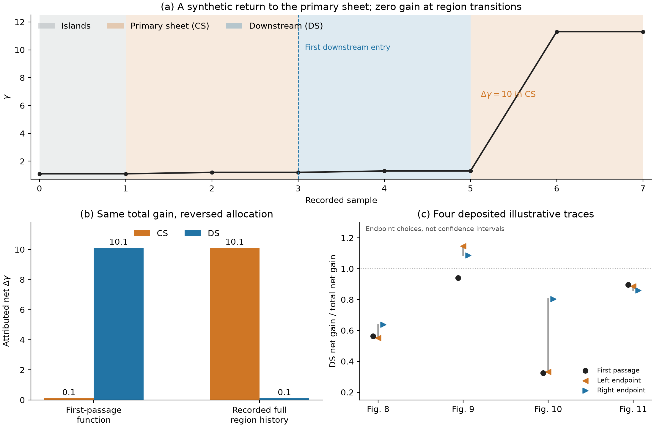
Its final Lorentz factor lies in the same intermediate interval used by the public script, . Every interval whose endpoint region labels differ has zero energy change. Consequently neither a choice of left versus right endpoint nor interpolation of a nonzero boundary increment explains the disagreement. The first-passage function returns
whereas summing increments over the recorded full region history gives
Both have total net gain , and all gains are nonnegative. The later sheet gain is assigned downstream by the first-passage definition. Scaling the nonzero gains by ten yields the same reversal in the high-energy branch: versus , with final . Two additional tests put downstream gain before first sheet entry; the function assigns that gain to its initial-phase term. Monotone I-to-CS-to-DS positive controls pass in both energy-band branches. These are direct executions of the pinned public function on constructed inputs, not synthetic data presented as PIC output.
A recorded-history alternative and what it can certify
For a target region , let denote its indicator and . Two transparent recorded-history conventions are
The symbols L and U identify left- and right-endpoint rules; U is not being defined as an upper bound. If the recorded labels form an exhaustive exclusive partition, then each rule obeys exact net closure:
Their difference is localized to intervals with different endpoint labels:
It follows immediately that
For the more specific discrete model that allocates each interval's net increment between its two endpoint regions, write with . Then
Equivalently the interval is centered at with half-width . Because the may differ between intervals, the two aggregate endpoint values alone need not be the extrema of that net-allocation model.
These are algebraic statements about recorded increments, not certified bounds on continuous physical work. Unrecorded energy gain and loss within an interval, or visits to another region between equal endpoint labels, cannot be bounded by endpoint differences alone. To estimate , one needs a stated crossing-time prescription and adequately resolved work/region histories, with a cadence study or independently justified assumptions. Reporting endpoint alternatives and net-allocation ranges exposes ambiguity; it does not make either alternative the uniquely corrected physical answer.
Reproducing the four published examples
The four preserved numeric fixtures contain 40,764 recorded samples each.
They retain the source values, shapes and dtypes, with hashes in
data/upstream-cc0/provenance.json, and are loaded without pickle. The pinned
function gives the following results; values in the code columns are shown to
six decimal places, while the printed columns reproduce the original panel annotations.
| Original figure | Printed CS | Code CS | Printed DS | Code DS |
|---|---|---|---|---|
| 8 | 2.33 | 2.325038 | 4.26 | 4.257615 |
| 9 | 0.00 | 0.000000 | 14.01 | 14.008444 |
| 10 | 64.49 | 64.494324 | 30.80 | 30.796448 |
| 11 | 3.51 | 3.514739 | 47.34 | 47.344337 |
All eight values agree after rounding to two decimal places. Reentry also occurs in these data: the histories corresponding to Figs.8, 10 and 11 have 15, five and 24 sheet-labelled samples after first downstream entry, respectively. The net increments with both endpoints in the sheet after that entry are approximately , and . The first-passage downstream term includes those later intervals irrespective of their recorded sheet labels. The sign can be positive or negative, so a direction of population bias does not follow simply from the function structure.
The following downstream values illustrate the finite-cadence distinction:
| Original figure | First-passage DS | Left endpoint DS | Right endpoint DS |
|---|---|---|---|
| 8 | 4.257615 | 4.176339 | 4.830590 |
| 9 | 14.008444 | 17.062301 | 16.171096 |
| 10 | 30.796448 | 31.566879 | 76.442074 |
| 11 | 47.344337 | 46.764732 | 45.434556 |
These values can exceed a particle's total net gain if another region has net cooling. Large differences between endpoint rules, especially in the Fig.10 trace, show why a single endpoint convention must not be advertised as a resolved continuous channel partition. The examples were selected by the authors for illustration. They neither represent an unbiased cohort sample nor determine the size or sign of a change to the published population mean.
Particle-mean and energy-weighted fractions
The script confirms a second, separate interpretive distinction. It reports , where is the particle's total net gain. This expression is mathematically well-defined when each denominator is nonzero; the inspected routine does not explicitly filter zero denominators. It pools sheet plus island contributions in the orange series. This is a valid particle-mean fraction. It is generally different from the aggregate energy fraction . For equal statistical weights and nonzero mean total gain,
Three equal-weight particles with gains and downstream fractions have a particle mean of but an aggregate downstream energy fraction of . Starting at , their final kinetic energies all lie inside the reported intermediate band. This example does not make the reported mean an incorrect estimator: it delineates which quantity it estimates. Unequal macro-particle statistical weights require the corresponding weighted definitions.
Scope of the correction
The direct reproducible result is a diagnostic-definition mismatch for general region histories, not a demonstration that downstream acceleration is absent. The original temporal and spatial dissipation diagnostics provide separate evidence of downstream activity, and the four particle examples retain nonzero downstream gains under the displayed alternatives. The public decks also positively resolve the printed field-coordinate and guide-profile ambiguities, and the region code explicitly subtracts the expanded sheet mask from island and downstream masks. Those checks should be credited.
A supported revision would either label the reported particle quantities as first-passage-phase gains, with a justified connection to the intended regional claim, or recompute full-history regional work with a documented cadence and crossing convention. It should distinguish particle-mean fractions from total energy shares and show the separate island contribution when claiming primary sheet dominance. The current evidence does not quantify the full-cohort change, establish a sign for that change, overturn the paper's main downstream trend, or certify any uniquely corrected continuous physical partition.
5. Matched attribution on the released particle batches
Available cohort and paired analysis
The public deposit permits a larger empirical comparison than the four
illustrative traces. We retrieved all 32 files in its two released
trajectory batches, verifying each file's source SHA256 and byte count
before starting the next transfer. These comprise 517 histories in
inter_energy/p008 and 486 in high_energy/p000, each with 40,764 saved
samples. The batches have stable, unique integer tracer IDs in the same
order across all eight time chunks, and their ID sets are disjoint.
The 17-channel tracer arrays have shape (17, time, particle); the
separate region arrays have shape (time, particle). Their region
values are integer labels 1--5 stored in float64 arrays. The ID channel
is not a charge or statistical weight.
We concatenate the individual histories before applying the source's strict final- cuts, as its analysis driver does. The folder names are staging groups, not the final physical energy bands. Of the 1,003 released histories, 667 satisfy and 84 satisfy ; the remaining 252 lie below the lower cutoff. None equals either boundary. The intermediate staging folder contributes 265 intermediate-band histories and 252 exclusions; the high staging folder contributes 402 intermediate-band histories and all 84 high-band histories. Folder averages are not averaged together.
That composition can matter for extrapolation. Within the intermediate
band, the 265 p008 records have a downstream FP particle mean of
0.885079 and a symmetric mean of 0.916422, a paired increase of 3.13425
percentage points. The 402 records supplied by the high staging folder
instead have means 0.616068 and 0.541209, a paired decrease of 7.48594
points. The released union weights these observed groups by their record
counts, so their opposite shifts combine to the reported decrease of
3.26652 points. This is an observed mixture, not an estimate of the
mixture in the missing batches. The release may over- or underrepresent
particular energy ranges, initial locations or return histories; neither
its selection probabilities nor the missing conditional means are known.
No direction or size of a full-population bias follows from these group
comparisons. A resampling diagnostic conditional on the released records
also cannot repair an unknown release-selection mechanism.
The primary weights are explicitly unit empirical weights. The example
island deck assigns the same physical macro-particle weight = Np/Ne
to all tagged electron species, so those weights would cancel in the
within-batch fractions under that posted setup. Neither this fact nor
the filename batch indices establish archive inclusion probabilities.
The deposited driver loads intermediate batches 0--14 and high batch 0;
only intermediate batch 8 is publicly provided. The released union is
therefore an available subcohort, not an asserted probability sample or
a reconstruction of the entire Fig. 6 population. It contains
all eight time chunks of the released high staging p000 selected by
that posted driver. Its completeness relative to the historical
high-energy cohort is not established.
Every comparison uses the same selected IDs and the same denominator . The source first-passage calculation preserves the stored float32 values and its native arithmetic; the full-history left, right and symmetric calculations subtract and accumulate those same stored values in float64. They do not recompute the underlying Lorentz factors. On a fixed systematic selection of 32 histories per staging batch, the streaming first-passage outputs agree exactly with the pinned original function. Randomized branch/boundary checks, four source-linked fixtures and independent small-sequence checks additionally test the implementation. The largest source-arithmetic closure residual is ; the left and right ledgers have zero closure residual at the reported numerical precision.
The example linkage is also directly testable. All 40,764 stored and region values of the source's Figs. 9--11 match three columns of the high staging batch exactly, including their canonical-array digests. The Fig. 8 history was not found in either released batch. This ties the available files to three published examples; it does not identify all the historical plotting inputs. The arrays contain no timestamp channel. Filename ordering follows the posted loader, rather than independently verified physical time vectors.
Paired regional fractions and energy shares
For each convention we report both the mean particle fraction and the fraction of the selected histories' total net gain . All 751 selected histories have positive, finite, nonzero ; no denominator filter is active. Signed regional terms are retained. The JSON also records the original source's unfiltered denominator convention, in which three float32-derived phase terms stored in float64 arrays are summed; its small rounding differences do not change the table at six decimals.
| Available band | Convention | Mean particle DS fraction | DS share of total net gain |
|---|---|---|---|
| Intermediate () | First passage | 0.722947 | 0.679606 |
| Intermediate () | Left endpoint | 0.652728 | 0.597338 |
| Intermediate () | Symmetric | 0.690281 | 0.622373 |
| Intermediate () | Right endpoint | 0.727834 | 0.647409 |
| High () | First passage | 0.500318 | 0.490959 |
| High () | Left endpoint | 0.370742 | 0.377414 |
| High () | Symmetric | 0.370129 | 0.393724 |
| High () | Right endpoint | 0.369515 | 0.410033 |
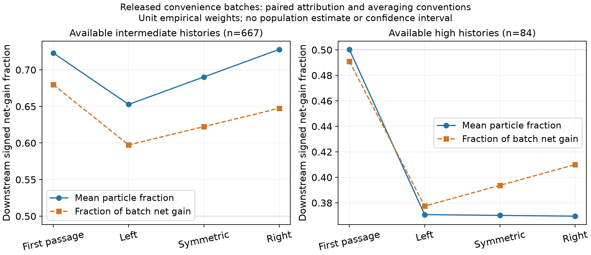
For the available intermediate histories, downstream remains larger than its signed non-downstream complement under every displayed convention. The empirical changes are nevertheless material: the mean fraction moves from 0.722947 to 0.652728 under the left rule, while the right rule gives 0.727834. Thus even the sign of the first-passage versus local difference depends on the declared sampling convention here.
For the 84 available high-band histories, the first-passage particle mean is only just above one half; all three full-history endpoint conventions give approximately 0.37. The aggregate energy-share estimand is already below one half for first passage, and ranges from 0.377414 to 0.410033 for the local conventions. The difference between the two estimands is therefore consequential even before attribution is changed. These are measured available-subcohort results, not a claim that the preprint's full-cohort ordering has been reversed.
The available intermediate first-passage mean, 0.722947, does not reproduce the preprint's displayed intermediate point (approximately 0.681). The available high-band first-passage mean agrees with the displayed high-band point at three decimals (0.500), which is useful consistency evidence but does not identify an exact historical cohort. We therefore distinguish the measured available union from a complete reconstruction of Fig. 6.
The full-history calculation retains IS1, IS2, top/bottom, downstream and primary sheet separately. Its actual CS+IS1+IS2 pool excludes top/bottom. The latter has a small signed intermediate-band mean fraction, from for the left rule to for the right rule, and zero in the available high band. The separately reported all-non-downstream complement includes top/bottom. Neither pool is silently identified with the source's CS+chronological-residual phase quantity.
Returns, signed increments and limits
Among the selected histories, 187 of 667 intermediate particles and 40 of 84 high-band particles visit the primary sheet after their first downstream sample following first sheet entry. There are respectively 743 and 89 subsequent sheet-entry events. The total numbers of recorded region transitions are 51,156 and 6,976, and the sums of absolute net increments on label-changing intervals are 10,974.343544 and 2,264.209734. These are discrete transition diagnostics, not bounds on unresolved continuous work.
Negative regional net gains are not discarded: the left rule gives 79 intermediate and 18 high histories with negative downstream net gain. Fractions above one also occur because a different region can supply a loss. Both features are compatible with total-gain closure; clipping them would change the estimands. Per-particle arrays, gross positive/negative recorded increments and all per-folder subsets are retained in the accompanying numeric outputs.
This comparison quantifies the attribution difference on every released history that meets the source cuts, rather than on a newly selected illustrative set. The omitted intermediate batches, uncertain archive selection, coarse region sampling and absent timestamps still prevent a certified full-population correction or a unique continuous-work partition. A physical convergence study requires more information than the small endpoint-convention differences in one band. The repository provides an explicit public fetch command, the 32-file hash inventory, a memory-bounded analyzer and compact NPZ/CSV results; the 3.11 GB raw files remain outside the code archive.
Complete-function validation and conditional empirical resampling
We extended the source-function validation from the previous systematic 32-history check per staging batch to every released input history. The new validation rechecks the sizes and SHA-256 values of all 32 raw files, retains their filename-ordered time chunks, and assembles only the stored float32 Lorentz factors and losslessly converted integer region labels. These arrays occupy 204,431,460 bytes. The complete, unchanged 60-line function printed in Appendix D is then executed once on the pooled 1,003 histories, rather than only on the 751 histories selected beforehand. Its own strict final-energy tests select 667 intermediate and 84 high-band histories and exclude the remaining 252. Both returned index lists and all six returned regional-gain arrays agree exactly with the streaming results, with zero mismatching values and zero absolute difference. Thus the reported first-passage values are now validated by a direct complete-function execution on every selected history. The original module's unrelated top-level filesystem operations are not run.
The source returns float64 arrays containing differences calculated with the native float32 input arithmetic. Our comparisons use the common denominator evaluated in float64 from those same stored endpoints. Replacing that denominator by the source's sum of returned phase terms changes the downstream particle mean by in the intermediate band and in the high band. These small denominator effects are reported separately from the attribution differences; no higher-precision particle history is inferred.
To describe the dispersion under an explicit empirical resampling model, we also apply a paired history bootstrap [11]. Within each already selected energy band, each replicate draws the original number of complete history IDs with replacement and equal empirical probability. The same resampled IDs are used for first passage, all three full-history conventions and both estimands. Write for . For one resampled index list , the two paired differences are
Repeated IDs appear with their draw multiplicity. The ratio-of-sums denominator is recomputed from those same draws, rather than resampling numerators and denominators independently. All selected are positive; regional gains and differences remain signed. We use 20,000 replicates per band, seed 20261029, PCG64 with separately identified band streams, and 2.5th and 97.5th percentiles with NumPy's linear quantile rule. Computation uses blocks of 256 replicates without changing the resampling unit. The following values are changes from first passage, in percentage points.
| Available band | Convention | Particle-mean change | Conditional 2.5--97.5 percentile range | Total-net-gain-share change | Conditional 2.5--97.5 percentile range |
|---|---|---|---|---|---|
| Intermediate () | Left | -7.0218 | [-11.0001, -3.0968] | -8.2268 | [-12.0219, -4.5109] |
| Intermediate () | Symmetric | -3.2665 | [-6.3470, -0.2036] | -5.7232 | [-8.6783, -2.8621] |
| Intermediate () | Right | +0.4888 | [-4.3746, +5.8511] | -3.2197 | [-7.0472, +0.7179] |
| High () | Left | -12.9576 | [-22.0785, -4.4437] | -11.3545 | [-19.4089, -4.4561] |
| High () | Symmetric | -13.0189 | [-20.4864, -6.6663] | -9.7236 | [-17.2950, -3.3956] |
| High () | Right | -13.0803 | [-22.0611, -4.3208] | -8.0927 | [-17.5015, +0.9552] |
These are central 95% conditional iid empirical bootstrap percentile ranges, not population confidence intervals, significance tests or physical uncertainty bounds. The iid draws describe variation under the empirical distribution of the available histories. Archive release probabilities are unknown, so this procedure cannot account for selection into the public files. Particles from one simulation can also share structures and be correlated; resampling them as independent histories can understate uncertainty. Independent-run or defensible structure-cluster replication is not available here. The ranges do not cover temporal or mask cadence, hidden recrossings, unresolved electric work, alternative release compositions or omitted histories. In particular, an interval endpoint's position relative to zero is not presented as evidence of population-wide statistical significance. The high-band first-passage energy share was already below one half; these added diagnostics do not change that estimand distinction.
The portable script is
experiments/validate_full_source_and_bootstrap.py. After obtaining the
already documented raw cache, the new calculation is invoked as follows;
the command performs no download:
python experiments/validate_full_source_and_bootstrap.py --cohort-dir COHORT_DIRECTORY --output-dir NEW_DIAGNOSTIC_DIRECTORY
Choose a fresh output directory to retain the frozen published results.
The script writes newly named v1.2.0 validation, bootstrap JSON, replicate
NPZ and range-table CSV files, leaving the v1.1 outputs unchanged.
results/full-source-validation-v1.2.0.json records the full source execution
and raw-file bindings. results/paired-history-bootstrap-v1.2.0.json records
the resampling specification, percentile ranges and the hashes of all
replicate arrays and the full numeric table. Constant-shift, signed scalar
reference and block-size-invariance checks validate the paired implementation.
These remain computational checks, rather than independent human peer review.
6. Extending the comparison to the historical population
Section 5 executes the paired ledger comparison on all available posted histories and reports both estimands after common band selection. The remaining extension is to a completely identified historical Figure 6 cohort, with its run, endpoint, sampling design and physical weights. The following protocol specifies that extension and the separate validation of continuous electric work; it is not presented as an additional population calculation already completed here.
The demonstrated method discrepancy can be addressed without changing the underlying particle-in-cell calculation. The primary empirical question is how much the chosen regional statistic changes when the same cohort is analyzed with its full recorded region histories. Answering that question requires a matched comparison. Changing the cohort, energy cutoffs or masks at the same time would confound the attribution change with a different analysis selection.
The first step is to freeze the intended cohort. The report should identify the run, the final physical time associated with the chosen reconnected-flux fraction, the particle identifiers and the final-energy band. The source thresholds are stated in terms of , whereas the deposited routine accepts ; its intermediate-band inputs 5.77 and 16.40 correspond to 4.77 and 15.40 in the printed convention. The initialization tag, inclusion probability and macro-particle weight should be retained for each selected trajectory. A larger number of tracked samples alone does not establish that their distribution represents the entire target population.
The second step is to retain time and region information together. For each particle, record a monotone time vector, its energy samples and its region at each sample. Discontinuities arising from restarts, repeated output steps, particle sorting or chunk concatenation should be resolved explicitly rather than treated as physical acceleration. The full-history calculation should record the source of region labels and the mask update cadence, which may differ from the particle-output cadence. Where available, electric fields and velocities at the particle permit a separate electric-work quadrature check. That check should use the same units and temporal alignment as the energy record; it should not be replaced by an unrelated fluid-frame proxy.
Both the first-passage and full-history estimates can then be evaluated on exactly the same selected histories. The chronological estimate remains useful as an explicitly labeled transit-phase diagnostic. The full-history ledger should retain the two islands, top/bottom, primary sheet and downstream entries separately before forming any pooled quantity. This prevents a pooled sheet-plus-islands statistic from being interpreted as the primary sheet alone. Signed gains and losses should remain signed. Negative regional work, or a regional net contribution larger than the particle's total net gain, need not indicate failed energy conservation when another region supplies a loss.
Three validation levels should be distinguished. Algebraic closure checks whether all recorded increments have been assigned exactly once. Controlled one-pass and re-entry tests check the intended attribution semantics. Cadence and crossing tests assess how the recorded approximation approaches a physical work integral. Passing the first level cannot replace either of the others. The counterexamples in this audit are useful tests precisely because their total budgets close while their chronological and spatial meanings differ.
For a fixed sampling, reporting left, right and symmetric endpoint allocations exposes an important part of the observable ambiguity. The sum of absolute energy increments at changed endpoint labels gives a sensitivity budget for that restricted family of net-increment allocations. It does not cover hidden recrossings or work with cancelling signs inside an interval. A physical uncertainty claim therefore also needs finer sampling or directly integrated work with adequately resolved crossing information. The large convention differences in some selected examples motivate this check; they do not select one endpoint rule as the correct physical answer.
Finally, report the chosen population estimands and their denominators. The particle mean of regional fractions and the weighted fraction of total energy should be shown separately when both interpretations matter. If uncertainties are estimated, the sampling scheme and the correlations among particles in a common structure must be considered. Repeating a large number of correlated particle observations from one run is not equivalent to repeating independent simulation realizations. Sensitivity to the classifier's mixing threshold, sheet-width parameter and spatial expansion can be assessed as a separate postprocessing study, provided the necessary fields and tags are retained.
These steps define a concrete repair and comparison protocol. They do not predetermine whether the population-level correction will be small, large or of a particular sign. In particular, the separate positive reconstruction of the source's regional nonideal-work curves remains evidence for downstream activity under that diagnostic, regardless of the outcome of a particle-ledger reanalysis.
7. Limitations, reproducibility and disclosures
The source scope is the supplied 11-page arXiv:2511.15988v1, verified byte for byte against the official versioned PDF, together with explicitly dated and hashed files in the author-associated OSF deposit [2]. The current official arXiv record lists only v1. Our bounded checks did not identify a journal edition or erratum. Differently titled, unindexed or inaccessible versions remain possible. The OSF deposit has later updates and figure numbering that differs from the preprint; the entire deposit is not treated as a single historical snapshot of the preprint's execution.
The four trajectory examples were selected by the original authors for illustration. Three exactly match gamma, position and region histories in the larger public batch over all 40,764 samples. The revised analysis also includes every one of the 1,003 posted batch histories and applies common final-energy cuts after pooling; 667 intermediate and 84 high-energy records enter the main comparisons. Neither complete processing of these files nor their internal example matches establishes random release selection, inclusion probabilities or a revised full-population Figure 6 mean. The available intermediate-band first-passage mean differs from the published point. The high-band mean agrees only at three-decimal rounding. An exact historical cohort, its complete weights, every plotting operation and the executed simulation binary have not been identified. No claim of reversal of the full-cohort downstream/current-sheet ordering follows.
On 29 October 2026 at 19:58:41 UTC, Taylor Kalin sent a data and provenance request to Alexander Velberg at velberg@mit.edu for the omitted Figure 6 cohort histories, weights and analysis provenance. Dispatch was verified in the sender's Sent record; submissions/author-correspondence.json records the request. A reply and any additional data remain pending as of the recorded verification. Sending the request does not establish the historical cohort, receipt by the recipient or author endorsement.
The discrete full-history estimators retain all recorded visits and signed energy increments. Their left, right and symmetric endpoint conventions can differ considerably when energy changes during recorded transitions. Bounds among endpoint allocations do not bound true continuous work when there are unresolved crossings, returns or sign-changing work within a sample interval. A physical reanalysis should evaluate electric work together with sufficiently resolved position and region histories, test sampling cadence and mask choices, and report uncertainty. Our synthetic examples avoid this ambiguity by construction; the real examples do not.
Pooling the primary sheet with the islands is disclosed in the source Fig. 6 caption and implemented in the posted statistics. We retain the source phase pool as such and report actual CS-plus-islands and all-non-downstream pools separately. A particle-mean ratio is also a legitimate statistic. Its mathematical distinction from the share of total energy is not itself an implementation error. A complete population analysis should identify the chosen estimand, macro-particle weights and sample selection, and retain or explicitly account for negative net increments rather than silently clipping them.
The force-free field checks address the printed formula and posted example inputs. They do not establish that an erroneous field was used in the original calculation; the available code instead supports the corrected expression. Approximate grid-spacing language is resolved by the run information, including the stated number of particles per species. The caption exponent discrepancy is a local presentation inconsistency and does not establish an error in a fitted spectrum. We do not infer fabrication, misconduct, intent or failure of the reconnection mechanism from any of these observations.
The electron-frame diagnostic remains useful and Lorentz invariant as defined. Its distinction from a laboratory magnetic-energy budget is an established diagnostic issue, not a discovery that invalidates the source's proxy. The positive curve reconstruction is kept separate from any unresolved run alignment or velocity-file semantics. We have not established an erroneous implementation of that diagnostic or an incorrect normalization of the published curves. Such claims would require an identified producer, execution and plotting chain beyond a variable name or a raw-array comparison.
Code and data availability. The public repository is https://github.com/Teylersf/multiscale-reconnection-audit . Its computational snapshot e3119e6ee98f6d4bfc760a7c851d33f90b3a7d6b is archived as software version 1.0.0 at https://doi.org/10.5281/zenodo.23774456 [9]. This DOI identifies the code and data archive, not a paper acceptance. The repository contains this manuscript, original audit code, reproducible results and figures, exact upstream provenance and a small set of permitted CC0 fixtures. The default particle-attribution reproduction uses numeric-only NPZ arrays and a pinned excerpt of the deposited function. It does not execute the original script's top-level filesystem operations or load arbitrary object pickles. The analysis records the original and converted file hashes and per-array byte digests. The proxy reconstruction and analytic checks have separate scripts and results. All are designed to run from repository-local inputs; no original HPC path, GPU allocation or full particle-in-cell rerun is required. The release records exact scientific artifact hashes and separates venue receipts from numerical evidence.
The revised computational snapshot a8cb56dadaf6fdf6d07ce6aba0d94b9ad291f9d5 is archived as software version 1.1.0 at https://doi.org/10.5281/zenodo.23775167 [10], with direct record https://zenodo.org/records/23775167 . It adds the serialized public-data fetcher, streaming paired analysis, compact per-particle NPZ/CSV exports, independent summary verifier and all source-link receipts. The archive is 2,702,929 bytes, with SHA-256 82835a9d7e53c929a690cc5ccc30f3cfdc0efa75ea23344c9f6682ad737b421e. The 3,107,362,288 bytes of raw batch arrays are linked through their 32-file hash inventory rather than duplicated in this package. The software DOI is registered through DataCite; its primary registry record is https://api.datacite.org/dois/10.5281/zenodo.23775167 . Snapshot-bound checks of the compact exports need no network. A complete raw-data reproduction requires the explicit public download; fresh runtime metadata may differ from the frozen report's byte hash. No private data or author confirmation has been obtained for the unprovided historical cohort.
The additional complete-function validation and resampling diagnostics are archived as software version 1.2.0 [12], DOI https://doi.org/10.5281/zenodo.23777646 , direct record https://zenodo.org/records/23777646 . Its computational snapshot is 83660394cdbd789f297c6da5f18470c00942254a. The 4,542,752-byte archive has SHA-256 0398c88dc2a68471e283b75240d95235ad78bcc2f4f1946fcb814b3f966954fa. Newly named diagnostic outputs preserve all earlier versioned numeric evidence. A fresh output directory permits repetition without overwriting the frozen results.
For references [9] and [10], DOI resolution was verified directly on 29 October 2026. The DataCite record for [9] returned HTTP 200 and state findable at 18:26:49 UTC; its doi.org link resolved to Zenodo record 23774456 with HTTP 200 at 18:26:52 UTC. Reference [10] returned the same positive DataCite state at 19:12:20 UTC and resolved to record 23775167 at 19:12:22 UTC. The official doi.org registration-authority responses identify DataCite. Primary registry links are https://api.datacite.org/dois/10.5281/zenodo.23774456 and https://api.datacite.org/dois/10.5281/zenodo.23775167 . Timestamped receipts preserve these checks and anonymous archive hashes. Crossref not_found is not evidence that a separately verified DataCite DOI is invalid.
Authorship and assistance. Taylor Kalin is the canonical author and is responsible for this audit and its release. AI tools assisted with source retrieval, mathematical checks, code, internal adversarial review and drafting. These checks are not represented as independent human peer review. Separately authorized agent editions identify their agent byline and retain Taylor Kalin's human-operator and canonical-author credit when a venue requires agent authors.
Funding and interests. Taylor Kalin self-funded this study and reports no outside funding. No competing interests have been reported. The original authors, their institutions and the publishers have not endorsed this audit. Original audit text and figures are CC BY 4.0 and original code is MIT licensed. Upstream fixtures and code excerpts retain their CC0 provenance; other attributed excerpts retain their source rights. The original paper, complete source archive and large simulation outputs are linked rather than republished as this author's work.
Publication disclosure. Repository and preprint versions are identified separately from any venue review or acceptance; actual publication states are recorded in the accompanying receipts.
8. Conclusion
The deposited particle-analysis function calculates first-passage phases. For a trajectory that revisits a region, those phases need not identify the locations of its energy gains and losses. An exact counterexample changes the inferred dominant region while preserving total-gain closure, so closure alone cannot validate regional attribution. Four released trajectories reproduce the eight preprint annotations, and three match full histories in the larger released batch. The revised calculation measures the attribution difference on 751 in-band records selected from all 1,003 posted histories.
For the available high-energy subset, the downstream particle mean decreases from 0.500318 to 0.370129 under symmetric full-history attribution, a change of 13.0189 percentage points. Left and right conventions give similar high-band particle means, whereas the intermediate subset retains downstream dominance. The high-band fraction of total net gain decreases from 0.490959 to 0.393724; it was already below one half under first-passage attribution. Thus the two estimands must not be described as undergoing the same ordering change. These are measured paired effects with the available histories, not a uniquely recovered continuous-work partition or a correction to the complete published cohort. The mismatch to the original intermediate-band point and the undocumented batch-release selection keep that population question open.
Other checks preserve important positive evidence: the posted fields implement the correct initialization, the force-free guide profile is explicit in the input, and the reported nonideal-work curves can be reconstructed after their plotting transformations. The resulting correction is specific to what has been demonstrated. It calls for a more precise regional particle-energy attribution while retaining the physical results that this audit does not overturn.
Appendix A. Estimator identities and sampling limits
This appendix supplies self-contained proofs for the estimands used in the main comparison. Acceleration after downstream entry and acceleration while downstream coincide for a one-pass history, but need not coincide after re-entry. These are elementary bookkeeping identities, not new particle dynamics or new general dissipation laws.
First-passage epochs
Consider one particle with saved Lorentz factors and mutually exclusive region labels . Let denote the primary current sheet and the downstream region. If a sheet visit is followed by a downstream visit, define
The deposited function returns
Here is the routine's residual contribution, called islands in the code; the formula does not itself test whether every contributing sample is in an island. Band selection acts on the final energy and does not change these per-particle identities.
Proposition 1 (epoch interpretation). Put . The first-passage outputs are precisely the sums of over the chronological intervals , and , respectively. They therefore sum to , independently of the labels between the selected entries.
Proof. The three sums telescope to their stated endpoint differences. Their index intervals partition , so their sum telescopes again to the total change. No intermediate region indicator occurs.
In the other source branches, a particle that never visits is assigned a downstream epoch beginning at its first sample. If is visited but no later sample occurs, the sheet epoch runs from first to last sample, with the remainder assigned to . These are also chronological partitions; they need not follow each intervening region visit.
The first-passage calculation is a valid phase statistic. For a strictly ordered history whose saved labels remain in islands before , in from through , and in thereafter, it also equals a left-endpoint regional-increment sum. That is a sufficient condition, not a necessary condition: accidental cancellations can yield agreement for other histories. Total-gain closure alone cannot establish the condition.
Counterexample family and exact attribution discrepancy
Let be the gain in a first sheet visit, the gain downstream and the gain in a later sheet visit, with zero gains on the intervening transitions and no initial-phase gain. Such a history has saved labels ; starting at , its energies are . The first-passage and visit-local pairs are
Their downstream-share difference is . It approaches one as grows with fixed. For and , the outputs are and , both closing to 102. Left and right endpoint rules agree because every transition increment is zero. Smooth gain episodes supported inside constant-region visits give the same result, so the reversal does not depend on crossing-time tie breaking. It does not estimate the source cohort's error.
For an arbitrary saved history with downstream epoch beginning at , write for the left-endpoint regional sum defined below. Its exact discrepancy is
Thus non-downstream gains after first downstream entry and downstream gains before that entry contribute with opposite signs. With losses, island excursions and re-entry, there is no universal sign of the bias.
Full-history estimators and closure
For continuous collisionless Lorentz dynamics without additional forces, . A regional net-work target is therefore
The masks may move. This target describes changes in a particle's energy while in a region; it is not the energy carried into that region or stored there at the final time. If , summing over regions gives the total particle-energy change.
An explicit finite-cadence convention is
This uses every visit. A right-endpoint version uses instead. Both retain signed changes and all regions, including the two islands and top/bottom region even when some are later pooled for presentation. For one particle, the main text writes these two values as and ; the latter symbol denotes a right-endpoint rule, not an upper bound.
Proposition 2 (discrete closure). For any interval-allocation weights satisfying , define . Then
Proof. Interchange the finite sums, insert the unit sum of weights and telescope the increments.
Nonnegative allocation weights support the interpretation of assigning each interval to regions; the closure identity itself only requires their unit sum. A useful conservative output assigns intervals with equal endpoint labels to that label and places label-changing intervals in an explicit unclassified-transition category. The category must remain in the closure sum. Equal endpoint labels still do not exclude an unresolved exit and return within the interval.
Endpoint sensitivity is not a continuous-work error bound
For , consider the endpoint-allocation family
It contains left, right and symmetric endpoint assignments. These weights are bookkeeping choices, not inferred fractions of time spent in a region. Define the endpoint transition diagnostic
Proposition 3 (allocation sensitivity). For any two members of this family and any region,
Proof. Their per-interval difference is . It vanishes when the labels agree. Otherwise its absolute value for one region is at most , and its sum over region absolute values is at most . Apply the triangle inequality and sum.
There is a sharper, attainable per-region range within this allocation family. Set and . Then
or, equivalently, . To attain the lower or upper endpoint for this region, choose each as 0 or 1 according to the sign of . The choices can differ between intervals, so and need not be the extrema. Different regions' extrema need not occur for the same choices.
These bounds concern only the stated discrete allocation family. cannot generally bound the error relative to continuous regional work. For example, sample a particle downstream at both ends of one interval with the same energy. Between samples it can enter the sheet, gain , return downstream and lose . Its endpoint increment and are zero, while its regional net gains are in the sheet and downstream. Smooth gain/loss episodes can occur away from the crossings. Sign cancellations create a similar obstruction even in an interval with different endpoint labels.
For a left-endpoint assignment the continuous discrepancy obeys the standard inequality
A useful physical bound needs information about the work rate and crossings on those intervals. Endpoint net increments do not supply its total variation. Recovering continuous regional work consequently requires adequate particle/field/mask cadence or pusher-level diagnostics, resolved crossings and a convergence check. Electric-work quadrature should also be compared with the numerical change in particle kinetic energy rather than assuming an exact identity for a finite-step pusher.
Particle averages, energy shares and signed gains
For one selected energy band, put and . First suppose for every included particle and their physical weights are equal. A mean particle fraction and a fraction of the band's total net gain are respectively
Proposition 4 (covariance distinction). With population covariance ,
Proof. Since , ; insert .
The mean particle fraction and energy share answer different questions, as the main text's within-band example demonstrates. The deposited code [2] explicitly uses the particle mean and pools current-sheet plus island contributions; that statistic should not be silently renamed an energy-weighted total partition. For unequal macroparticle weights , the same identity holds for the physical number-weighted mean and covariance defined using ; an unweighted macroparticle mean then needs separate justification.
Regional net gains can be negative even if , and individual fractions can lie outside . Clipping negative contributions changes both the estimand and the closure. If , its per-particle fraction is undefined; if signed total gains or a near-zero ensemble denominator are included, the ratios are not probability shares and may be poorly conditioned. Report these cases explicitly. Gross positive and negative work can be useful additional quantities, but neither is reconstructed by net endpoint changes alone. The selected final-energy band, sampling weights and masks must remain fixed and disclosed when comparing estimators.
Appendix B. Ancillary source and diagnostic checks
These checks separate local source-description issues from the regional attribution finding. They do not establish an erroneous VPIC evolution.
Printed equilibrium and the correctly posted field
Equation (1) of the preprint [1] prints , while and . Direct differentiation gives
At the origin this is for , so the printed field is not solenoidal. Replacing the numerator by restores the intended force-free modification of the Fadeev geometry [1,4]. In fact, with ,
The first two identities make the divergence zero; differentiating and the in-plane components gives the last identity, so . Force-free does not imply constant for this curved equilibrium: .
Both currently deposited example decks [2] use the corrected numerator for their unperturbed base field. The coalescence initialization also adds the documented triggering perturbation; the equilibrium identities above refer to the base field, not to that intentionally perturbed state. Their common guide-field prescription is
The coalescence example has . The force-free current-sheet example has and , hence . This is genuinely force-free with ; its total is . The preprint's footnote [32] describes replacing the out-of-plane field by an external guide. Read literally as a uniform replacement, , it would instead give
which is nonzero. The posted profile resolves that description; it provides a positive code check rather than evidence of a force-free implementation failure. Present deposited examples and metadata do not independently identify the exact historical binary and inputs for every reported run.
Spectral caption
The body and inset of Fig. 5 in [1] specify a power-law index near 3.3, while the caption specifies 3. The caption should identify the plotted guide consistently. This local discrepancy does not establish a different fitted exponent, invalidate the ankle, or reproduce the spectral fitting procedure.
Electron-frame nonideal work and laboratory energy
The electron-frame measure used in [1] is the established relativistic nonideal-work diagnostic [3]. Once the physical electron flow is specified, is Lorentz invariant; it should not be described as observer-frame dependent. Its relation to the laboratory work rate is the standard identity, in dimensional Gaussian units,
The second equality follows by the scalar triple-product identity. It is not a new dissipation law. Poynting's theorem instead gives
Thus an integral of normalized by initial magnetic energy is a normalized nonideal-work diagnostic, not by itself an exact magnetic-energy loss or irreversible heating fraction [3,8]. The paper explicitly calls it a proxy. Its reported regional ordering is not disproved by this distinction. The posted Python expression is consistent with the normalized convention. This dimensional identity does not identify a unit error in the published diagnostic outputs.
A portable exact check illustrates the distinction. In normalized units, homogeneous cold counterstreaming beams with momenta satisfy and . A parallel constant magnetic field does no work and does not change. The conserved electric-plus-particle energy is . From to the first , , the laboratory field-energy loss and particle-energy gain are both 0.5, whereas . This checks the lack of a general equality; it is not a reconnection simulation or an estimate of the diagnostic bias in [1].
Finally, implementation requires the physical definition and producer of any input velocity/momentum files and the order of temporal averaging. Variable names alone do not establish that a mean particle proper momentum is the four-velocity of the number-flow mean. Those semantics remain a reproducibility limitation here; no unverified velocity-file bug is claimed.
Appendix C. Positive checks and inferred display reconstruction
The proxy arrays require the same care. Their raw L320 time series has 122 entries ending at 23.16347, while its raw cumulative total reaches 0.357089. Directly comparing those raw numbers with the preprint axes or with global magnetic-energy loss would suggest a large discrepancy. We therefore extracted numerical line coordinates from the original vector figures in the official v1 source archive and calibrated their axes. This checks the displayed data rather than guessing the missing plotting convention.
The following display factors and filter are inferred reconstruction conventions, not independently identified historical plotting instructions. All five cumulative L320 curves in preprint Fig. 3 are reproduced by the first 116 deposited samples using
The island curve uses the sum of the two deposited island arrays.
There is source-code unit corroboration for these two scale factors,
independent of the coordinate fit. The posted tracer plotting driver uses
and , hence
in its plasma-frequency convention, and explicitly divides
its cyclotron-clock intervals by . The dissipation producer
instead records its raw cyclotron clock divided by . Conversion to
the stated plasma clock supplies the factor . For the nominal L320
output interval its raw cumulative multiplier is 4000, while the
corresponding plasma-time interval is 160, giving .
The scripts and exact line locators for this dimensional check are
recorded in data/source-claim-evidence.json. This corroborates the
scale conversion under the posted conventions; it still does not recover
a hash-identified original plotting execution. No matching posted
instruction for the Gaussian width below has been found.
At the common endpoint the reconstructed total is 0.0139557484 at , matching the published curve rather than the raw 0.357089 endpoint outside that window. Across the five cumulative paths and the rate reconstruction below, the largest coordinate residual is 0.000555 PDF point, smaller than the declared 0.002-point rounding tolerance. The original artwork is not redistributed; the portable artifact preserves attributed numeric coordinates and their source hashes.
The instantaneous and cumulative files are also coherent. Their stored increments obey with maximum absolute residual , consistent with float32 storage of the instantaneous array. The paper's relativistic Alfvén definition gives in plasma-time units for this case. Taking the first 115 instantaneous samples, applying a Gaussian filter of width 1.5 samples with half-sample symmetric boundary handling, and multiplying by reproduces the Fig. 4 blue rate path. The corresponding times are . This is an independently verified display reconstruction; it does not claim recovery of an unavailable historical plotting revision.
The common cumulative scale factor cancels in every regional share. At the displayed endpoint the downstream fraction is 0.664435 and the primary-sheet fraction 0.266235; the islands and top/bottom contribute 0.0586225 and 0.0107092. Those values are unchanged by the factor of 25. Thus the deposited curves positively preserve the preprint's downstream-dominant ordering of this proxy. They provide no basis for alleging that its published integral is too large by that factor. The independently generated reconstruction figure and executable check make this positive result reviewable.
The global-energy file supplies a bounded cross-check, not an identity between the proxy and magnetic-energy conversion. Its 2618 rows contain 102 repeated restart steps. Keeping either the first or last value at each recorded step gives identical data at the reported precision and 2516 uniformly spaced unique records. Matching the L320 timing conditionally, the endpoint of the published window gives an electromagnetic-energy loss of approximately and a rescaled integral of . These comparable values involve different averaging and output cadences and do not prove complete run identity or exact energy closure. The same conditional comparison gives a particle kinetic-energy gain of and a total recorded-energy change of . We report that residual without diagnosing its cause or claiming complete conservation from the comparison. The diagnostic spacing inferred from 409 simulation steps, five output intervals and the recorded timestep is 159.70949 plasma-time units; the displayed convention uses the nominal value 160, a 0.1819% difference. We record that distinction without converting it into an unsupported scientific-error claim.
Finally, this successful reconstruction does not identify with a magnetic-energy decrease or particle-energy gain. The electron-frame quantity is a useful proxy whose relationship to those budgets requires the appropriate work and transport terms. The narrower diagnostic-interpretation question remains legitimate, as do the separately tested particle-attribution questions. The published proxy normalization, however, is consistent with the available source arrays after their explicit display transformations.
The coordinate agreement tests whether the released arrays can reproduce the published paths under these explicit transformations. It does not uniquely identify why the original plot used a given scale, which revision of the plotting program was executed, or whether an equivalent historical pipeline used different intermediate units. In particular, the factor 25 is not reported as a discovered normalization error, and the inferred Gaussian filter is not presented as a documented instruction by the source authors. The dimensionless regional shares are invariant to a common positive cumulative scale. The numerical reconstruction is sufficient for that positive comparison; stronger producer provenance is a separate claim.
Appendix D. Deposited first-passage routine
The following is the complete unmodified function at lines 344-403 of the
December 6, 2025 version-1 OSF file python_scripts/tracer_functions.py [2].
The parent file SHA-256 is
3f93e1685dd9664e279f8b14535d4ebc6ba2946442e4831f4eaf24db315d61ba;
the exact 60-line excerpt SHA-256 is
2909f9e6acec3c48f3838e86c15ffd18a9563dc57984e400b0baadd22f16655f.
Its CC0 provenance, stable file identifiers and numeric-fixture conversions
are recorded in the reproducibility package. The original routine expects
NumPy as np and a tqdm iterator in its surrounding module; the audit harness
supplies these without executing the original module's top-level I/O.
Line labels in the typeset listing refer to the parent-file line numbers.
def get_energy_by_region_w_bands(gamma_data,region_data,separator1,separator2): # separator 1, 2 interms of gamma, not gamma-1
    npart = len(gamma_data[0,:])
    dgamma_cs_1 = np.zeros(npart)
    dgamma_ds_1 = np.zeros(npart)
    dgamma_isls_1 = np.zeros(npart)
    dgamma_cs_2 = np.zeros(npart)
    dgamma_ds_2 = np.zeros(npart)
    dgamma_isls_2 = np.zeros(npart)
    idx_1 = np.array([], dtype=int)
    idx_2 = np.array([], dtype=int)

    for i in tqdm(range(npart), desc="Processing particles"):
        gamma = gamma_data[:,i]
        region = region_data[:,i]


        if gamma[-1] < separator2 and gamma[-1] > separator1 :
            idx_1 = np.append(idx_1,int(i))
            # Now check if transits current sheet
            if len(np.where(region[:]==5)[0]) > 0:
                cs1 = np.where(region[:]==5)[0][0]
                cs_last = np.where(region[:]==5)[0][-1]
                if len(np.where(region[cs1 + 1:]==4)[0]) > 0:
                    ds1 = np.where(region[cs1 + 1:]==4)[0][0] + cs1+1
                    dgamma_cs_1[i] = gamma[ds1] - gamma[cs1]
                    dgamma_ds_1[i] = gamma[-1] - gamma[ds1]
                    dgamma_isls_1[i] = gamma[cs1] - gamma[0]
                else:
                    dgamma_cs_1[i] = gamma[cs_last]-gamma[cs1]
                    dgamma_isls_1[i] = gamma[cs1] - gamma[0] + (gamma[-1]-gamma[cs_last])
            elif len(np.where(region[:]==4)[0]) > 0:
                ds1 = np.where(region[:]==4)[0][0]
                dgamma_ds_1[i] = gamma[-1] - gamma[ds1]
                dgamma_isls_1[i] = gamma[ds1] - gamma[0]
            else:
                dgamma_isls_1[i] = gamma[-1] - gamma[0]
                print(i)
        elif gamma[-1] > separator2:
            idx_2 = np.append(idx_2,int(i))
            # Now check if transits current sheet
            if len(np.where(region[:]==5)[0]) > 0:
                cs1 = np.where(region[:]==5)[0][0]
                cs_last = np.where(region[:]==5)[0][-1]
                if len(np.where(region[cs1 + 1:]==4)[0]) > 0:
                    ds1 = np.where(region[cs1 + 1:]==4)[0][0] + cs1+1
                    dgamma_cs_2[i] = gamma[ds1] - gamma[cs1]
                    dgamma_ds_2[i] = gamma[-1] - gamma[ds1]
                    dgamma_isls_2[i] = gamma[cs1] - gamma[0]
                else:
                    dgamma_cs_2[i] = gamma[cs_last]-gamma[cs1]
                    dgamma_isls_2[i] = gamma[cs1] - gamma[0] + (gamma[-1]-gamma[cs_last])
            elif len(np.where(region[:]==4)[0]) > 0:
                ds1 = np.where(region[:]==4)[0][0]
                dgamma_ds_2[i] = gamma[-1] - gamma[ds1]
                dgamma_isls_2[i] = gamma[ds1] - gamma[0]
            else:
                dgamma_isls_2[i] = gamma[-1] - gamma[0]
                print(i)

    return dgamma_cs_1[idx_1], dgamma_ds_1[idx_1], dgamma_isls_1[idx_1],dgamma_cs_2[idx_2], dgamma_ds_2[idx_2], dgamma_isls_2[idx_2],idx_1,idx_2
The unused cs_last value in the downstream branch does not alter that
branch's first-passage definition. Branches for no subsequent downstream
visit and no sheet visit are preserved here; they are not replaced by the
simplified two-passage formula used in the main counterexample. The
routine's exact threshold comparisons and original return ordering are
also retained. Printing this later deposited version does not establish
that these exact source bytes were executed before the v1 preprint.
References
[1] A. Velberg, A. Stanier, X. Li, F. Guo, W. Daughton and N. F. Loureiro, Effects of Multi-scale Coupling on Particle Acceleration and Energy Partition in Magnetic Reconnection, arXiv:2511.15988v1 (20 November 2025). https://arxiv.org/abs/2511.15988v1 ; https://arxiv.org/pdf/2511.15988v1 . Audited preprint, including its supplemental material.
[2] A. Velberg, Effects of Multi-scale Coupling on Particle Acceleration and Energy Partition in Magnetic Reconnection, OSF code and data project. https://doi.org/10.17605/OSF.IO/EPWTU ; https://osf.io/epwtu/ . Specific file versions and checksums, rather than an undifferentiated project timestamp, identify the analyzed artifacts; accessed 29 October 2026.
[3] S. Zenitani, M. Hesse, A. Klimas and M. Kuznetsova, New Measure of the Dissipation Region in Collisionless Magnetic Reconnection, Physical Review Letters 106, 195003 (2011). https://doi.org/10.1103/PhysRevLett.106.195003 ; https://arxiv.org/abs/1104.3846 .
[4] V. M. Fadeev, I. F. Kvabtskhava and N. N. Komarov, Self-focusing of local plasma currents, Nuclear Fusion 5, 202-209 (1965). https://doi.org/10.1088/0029-5515/5/3/003 . Historical configuration cited by the source preprint; the force-free modification used here is checked directly.
[5] O. French, F. Guo, Q. Zhang and D. A. Uzdensky, Particle Injection and Nonthermal Particle Acceleration in Relativistic Magnetic Reconnection, The Astrophysical Journal 948, 19 (2023). https://doi.org/10.3847/1538-4357/acb7dd ; https://arxiv.org/abs/2210.08358 .
[6] R. Bird, N. Tan, S. V. Luedtke, S. L. Harrell, M. Taufer and B. Albright, VPIC 2.0: Next Generation Particle-in-Cell Simulations, IEEE Transactions on Parallel and Distributed Systems 33, 952-963 (2022). https://doi.org/10.1109/TPDS.2021.3084795 ; https://arxiv.org/abs/2102.13133 .
[7] Y. Yang, S. Adhikari and W. H. Matthaeus, Electron Dissipation and Electromagnetic Work, Journal of Geophysical Research: Space Physics 129, e2024JA033105 (2024). https://doi.org/10.1029/2024JA033105 .
[8] O. Pezzi, H. Liang, J. L. Juno, P. A. Cassak, C. L. Vasconez, L. Sorriso-Valvo, D. Perrone, S. Servidio, V. Roytershteyn, J. M. TenBarge and W. H. Matthaeus, Dissipation measures in weakly collisional plasmas, Monthly Notices of the Royal Astronomical Society 505, 4857-4873 (2021). https://doi.org/10.1093/mnras/stab1516 ; https://arxiv.org/abs/2101.00722 .
[9] T. Kalin, Computational evidence for First-passage attribution and regional particle energization in multiscale reconnection, version 1.0.0, Zenodo (2026), software and data. https://doi.org/10.5281/zenodo.23774456 . Computational snapshot e3119e6ee98f6d4bfc760a7c851d33f90b3a7d6b.
[10] T. Kalin, Computational evidence for First-passage attribution and regional particle energization in multiscale reconnection, version 1.1.0, Zenodo (2026), software and data. https://doi.org/10.5281/zenodo.23775167 ; https://zenodo.org/records/23775167 . Revised computational snapshot a8cb56dadaf6fdf6d07ce6aba0d94b9ad291f9d5.
[11] B. Efron, Bootstrap Methods: Another Look at the Jackknife, The Annals of Statistics 7(1), 1-26 (1979). https://doi.org/10.1214/aos/1176344552 .
[12] T. Kalin, Computational evidence for First-passage attribution and regional particle energization in multiscale reconnection, version 1.2.0, Zenodo (2026), software and data. https://doi.org/10.5281/zenodo.23777646 ; https://zenodo.org/records/23777646 . Computational snapshot 83660394cdbd789f297c6da5f18470c00942254a.