Introduction

A fundamental question in reinforcement learning is: how much of the world does a bounded agent need to model? For agents acting under partial observability, a natural answer is the Myhill–Nerode quotient of the history space under a fixed behaviour policy: two histories are equivalent if they induce the same distribution over futures. Nixon (2026b) develops this theory for bounded agents and Nixon (2026a) uses the resulting quotient to define a critical communication rate $R_{\rm crit}$ for multi-agent coordination. A companion paper (Pow 2026) gives a model-free estimator for finite observation–action alphabets: a permutation G-test on continuation histograms decides, for each pair of observed histories, whether their $k$-step continuation distributions differ, and a union–find pass merges the pairs that do not; the required number of trajectories is $N=O(|\mathcal{C}|\,n^2k\tau\log(n/\delta)/(T\varepsilon_{\min}^2))$ where $|\mathcal{C}|$ is the continuation alphabet.

The gap: continuous spaces, and what is not new.

Real POMDPs—manipulation, locomotion, audition—have continuous observation and action spaces. Applying the finite estimator requires discretising $\mathcal{O}\times\mathcal{A}$ into an alphabet $\mathcal{C}$, which (1) makes $|\mathcal{C}|$ grow exponentially in the dimension and (2) conflates continuation distributions that differ only within a cell. Both pathologies are visible in our experiments: a 3-bin G-test never recovers the two Tiger classes and an 8-bin G-test over-splits the 4-state K-cycle into 8 classes (Table 7).

We do not claim to be the first to group continuous histories by their predictive distributions with kernel embeddings. The RKHS $\varepsilon$-machine of Brodu and Crutchfield (2022) already represents $\Pr(\text{future}\mid\text{past})$ as a point in an RKHS, observes that clustering algorithms for conditional distributions map to the RKHS setting by using the MMD test, and recovers causal states by diffusion-map coordinates and clustering; causal-state learning (Zhang et al. 2019) approximates the same partition with recurrent predictors and discretisation; and bisimulation metrics (Ferns et al. 2011) address brittleness of exact equivalence in continuous state spaces. What those methods do not supply is an explicit finite-sample estimand with an analysed sample bound: the RKHS $\varepsilon$-machine and causal-state learning cluster point estimates with a user-set scale or threshold, and (to our knowledge) none of the cited methods states the partition that is recovered at a given sample size or a trajectory bound for it. Two-sample testing itself is not new here: the RKHS $\varepsilon$-machine maps clustering to the MMD test, and Mixed LICORS (Goerg and Shalizi 2013) permits nonparametric two-sample tests of equality of predictive distributions. Section 2 and the head-to-head comparison in Section 5.6 make the relationship precise.

Our contribution (restated).

We compare bin-conditional continuation laws with a kernel MMD permutation test on raw continuation vectors (Gretton et al. 2012), so no discretisation of the continuation space is needed, and key histories by coarse quantile bins so that enough continuations accumulate per key. The contribution is a finite-sample formulation of continuous quotient learning (an explicit estimand and an analysed sample bound for a pairwise-test estimator), not the idea of MMD- or test-based predictive-state clustering. Concretely:

1. Algorithm (Section 3). Quantile binning of the observation stream into $B$ bins, a biased-MMD$^2$ permutation test with a median-heuristic RBF kernel for every pair of bins, Benjamini–Hochberg (BH) control over pairs, and union–find merging.

2. What is estimated (Section 3). In continuous spaces the exact continuation-equivalence quotient of the history space is generically infinite (every observation value induces a different posterior), so we define the estimator’s target as the bin-level quotient $\mathcal{Q}^*_B$—the partition of the $B$ bins by equality of their bin-conditional continuation laws—and give conditions (bounded-support noise, bin edges aligned with class boundaries) under which $|\mathcal{Q}^*_B|$ equals the latent index $n$ (Proposition 1).

3. Alphabet-free sample complexity (Section 4). Using the concentration of the biased MMD statistic (Gretton et al. 2012, Thm. 7, Cor. 9) we prove that $N=O(B\log(B/\delta)/\varepsilon_{\mathrm{MMD}}^2+B^2\log(1/\delta))$ trajectories suffice to recover $\mathcal{Q}^*_B$ with probability $1-3\delta$ under the analysed variant (one window per trajectory; $\ell=1$, quantile bins; $B=K_{\mathrm{hist}}=O(n)$ in all our experiments). The $|\mathcal{C}|$ factor of the finite bound disappears; the dimension enters only through $\varepsilon_{\mathrm{MMD}}$. The theorem is about the analysed variant (T) (fixed kernel and bins, one window per trajectory sampling the exact pooled bin law, analytic threshold), not about the permutation/BH procedure used in most experiments; Section 4.1 states which guarantee applies to which procedure and Section 5.5 reports the experiments run under (T).

4. Resolution analysis. Because a two-sample test with $m$ samples cannot detect MMD gaps below $\approx\sqrt{\log(1/\alpha)/m}$, the finite-sample estimate is the quotient at that resolution: same-class bins whose laws differ slightly are merged, and distinct latent classes are separated only if their gap exceeds the detection scale. This explains all of our empirical findings, including the successes (aligned $B{=}n$) and the failures (over- and under-splitting at $B{=}2K$).

5. Experiments (Section 5). Ground-truth recovery on Tiger, K-cycle and a Gaussian-mixture random walk (90/90 at $B{=}n$), sensitivity to $B$ and $N$, partition-level accuracy (adjusted Rand index against the latent state) under $B$-selection rules that do not use $n$, runs under the analysed variant (T), a head-to-head comparison with an RKHS $\varepsilon$-machine, causal-state learning, a bisimulation metric, multivariate Wasserstein and DBC baselines, PO-MuJoCo, and end-to-end $R_{\rm crit}$ estimation on Dec-Tiger and a 4-state chain Dec-POMDP. All numbers are computed from result files released with the code (https://github.com/npow/quotient-learning-papers, directory cql/, artifacts at tag v1 = commit 83f9f42, new files in commit 2c16829; file list in Appendix E); every seed is reported.

Paper organisation.

Section 2 surveys related work; Section 3 defines the target and the algorithm; Section 4 states the guarantees; Section 5 presents experiments; Section 6 discusses limitations; Section 7 concludes. Proofs and full experimental specifications are in the appendices.

Related Work

PAC learning in POMDPs.

Observable operator models (Jaeger 2000), spectral methods for predictive state representations (Boots et al. 2011) and tensor methods (Azizzadenesheli et al. 2016) estimate latent dynamics with sample-efficiency guarantees when the number of latent states (or Hankel rank) is known. Our approach is model-free and targets only the quotient partition.

Predictive-state clustering with kernels (closest prior work).

Computational mechanics defines causal states as classes of predictively equivalent histories. Brodu and Crutchfield (2022) give the RKHS $\varepsilon$-machine: conditional distributions of the future given the past are embedded as points $\hat s_{Y|X=x}=\sum_i\omega_i(x)k^Y(y_i,\cdot)$ with regularised weights $\omega(x)=(G^X+\varepsilon I)^{-1}K(x)$, the similarity matrix $G^S_{ij}=\langle\hat s_{Y|x_i},\hat s_{Y|x_j}\rangle$ is converted to diffusion-map coordinates, and causal states are read off by a clustering algorithm (DBSCAN in their experiments); they also estimate an evolution operator on the causal-state manifold. They explicitly note that earlier clustering algorithms for conditional distributions map to the RKHS setting “by using the MMD test instead of other statistical tests”. Jurgens and Brodu (2024) extend this with causal diffusion components. LICORS and Mixed LICORS (Goerg and Shalizi 2012, 2013) reconstruct predictive states of continuous-valued spatio-temporal data by nonparametric clustering of conditional predictive distributions, and kernel embeddings of predictive state representations (Boots et al. 2013) handle infinite observation and action sets. Relation to our work. Our estimator is in the same family (kernel comparison of conditional futures), so the idea is not new. The differences are: (i) we discretise the pasts into quantile bins and run a two-sample test per pair of bins with a stated level (as noted above, test-based merging of predictive states is not new: Mixed LICORS permits nonparametric two-sample equality tests), whereas the RKHS $\varepsilon$-machine smooths over individual pasts with a regularised conditional embedding and clusters with a user-set scale; (ii) we state the estimand for finite samples (the bin-level quotient $\mathcal{Q}^*_B$, Definition 4) and an analysed variant with a sample bound (Theorem 1), where the cited work gives consistency-style arguments and no sample-complexity statement to our knowledge; (iii) their emphasis is dynamics and prediction in the original data space, ours is a discrete partition that the $R_{\rm crit}$ theory consumes. We therefore compare empirically with an RKHS $\varepsilon$-machine pipeline in Section 5.6, specialised to one-observation pasts as in the rest of the paper; our implementation follows the estimator equations of Brodu and Crutchfield (2022) but is not their released code, and we do not tune it with the ground-truth index.

Causal-state learning with recurrent networks.

Zhang et al. (2019) approximate the causal states of a POMDP (the coarsest partition of histories with identical conditional futures) with a recurrent encoder trained to predict the next observation and reward, and discretise the hidden states, e.g. by $k$-means. They prove connections to bisimulation metrics; the discretisation is not accompanied by a statistical test, so the number of classes is set by the discretiser (this concerns their recurrent-network pipeline only; test-based merging of predictive states exists in LICORS-type methods above). We compare against a GRU encoder with the same training signal and $k$-means (silhouette) discretisation. This baseline conditions on the full history, whereas our estimator uses one-step keys, so it is not handicapped by $\ell=1$.

Bisimulation and state abstraction.

Bisimulation relations (Larsen and Skou 1991) and bisimulation metrics (Ferns et al. 2004; Castro 2020) formalise (approximate) behavioural equivalence of MDP states and, for continuous state spaces, Ferns et al. (2011) show that the metrics are well defined and approximable by finite abstractions; Castro et al. (2009) extend these relations to partially observable MDPs. The brittleness of exact equivalence under perturbation is the classical motivation for metrics (Ferns et al. 2004). Deep Bisimulation for Control (DBC) (Zhang et al. 2021) learns metric-respecting representations from rewards and a learned latent dynamics model; bisimulation is reward-defined, so in the reward-free benchmarks of Section 5 we must supply a reward proxy (Section 5.6). Abel et al. (2020) analyse approximate state abstractions and their value loss. Our object is different: we cluster observed histories under a fixed policy, we output a discrete partition (which is what the $R_{\rm crit}$ theory of Nixon (2026a) consumes), and—in line with the bisimulation-metric literature—we make explicit that in continuous spaces the exact partition is generically infinite and what is recovered is a partition at a resolution set by the binning and the test.

Policy dependence.

The estimated quotient is the fixed-policy continuation-equivalence partition; under a random policy it may be trivial ($n{=}1$) and under a structured policy non-trivial. This is by design: the quotient characterises the agent’s minimal perception relative to its behaviour policy (Nixon 2026b).

Two-sample kernel testing.

The MMD (Gretton et al. 2012) is a nonparametric two-sample statistic that is consistent against all alternatives for characteristic kernels; permutation calibration gives exact finite-sample level. Block estimators (Zaremba et al. 2013) trade variance for $O(m)$ cost; we use the biased $O(m^2)$ estimator with at most $m_{\max}=300$ samples per side. Ramdas et al. (2015) show that with a fixed (e.g. median-heuristic) kernel the MMD separation between fixed alternatives typically decreases with dimension; this is why our bound is “alphabet-free” rather than “dimension-free” (Remark 2).

Method

Problem Formulation

Definition 1 (Continuous POMDP). A continuous POMDP is a tuple $(\mathcal{S},\mathcal{O},\mathcal{A},T,R,\Omega,\gamma)$ with $\mathcal{O}\subseteq\mathbb{R}^{d_O}$, $\mathcal{A}\subseteq\mathbb{R}^{d_A}$ (or a finite set), transition kernel $T:\mathcal{S}\times\mathcal{A}\to\Delta(\mathcal{S})$, emission kernel $\Omega:\mathcal{S}\to\Delta(\mathcal{O})$, reward $R$ and discount $\gamma$.

Definition 2 (Continuation law). Fix a behaviour policy $\pi$ and a window $k\ge1$. For a history $h=(o_1,a_1,\dots,o_t)$ the $k$-step continuation law $P^{(k)}_{h,\pi}$ is the law of $c=(o_{t+1},a_{t+1},\dots,o_{t+k})\in\mathbb{R}^{d_c}$, $d_c=k\,d_O+(k{-}1)d_A$, obtained by executing $\pi$ from $h$.

Definition 3 (Continuation-equivalence quotient). $h_1\sim_{\pi,k}h_2$ iff $P^{(k)}_{h_1,\pi}=P^{(k)}_{h_2,\pi}$. The quotient $\mathcal{Q}^*_{\pi,k}=\mathcal{H}/{\sim_{\pi,k}}$ has index $n=|\mathcal{Q}^*_{\pi,k}|$. We say the POMDP has finite latent index $n$ if there is a class map $c:\mathcal{H}\to[n]$ with $P^{(k)}_{h,\pi}=P^{(k)}_{c(h)}$.

Remark 1 (Exact quotients are generically infinite in continuous spaces). If the emission kernel has a density with unbounded support (e.g. Gaussian noise), the posterior over the latent state given a history varies continuously with the observed values, and so does the continuation law; hence $\mathcal{Q}^*_{\pi,k}$ is uncountable and the latent index is not the history quotient index. For instance, in Tiger with $o=\pm1+\mathcal N(0,\sigma^2)$ and one-step histories, $P(\text{Right}\mid o)=\mathrm{logistic}(2o/\sigma^2)$ and no two observation values share a continuation law. What a finite estimator can target is a quotient at a resolution, which we now define.

Coarse History Binning and the Bin-Level Quotient

Given $N$ trajectories we reduce each observation to a scalar $z(o)$ ($z(o)=o$ if $d_O=1$, else $z(o)=\|o\|_2$; the implementation exposes this map), fit $B$ equal-frequency (quantile) edges of $z$ over all time steps, and key a history of length $\ell$ by the tuple of bin indices of its last $\ell$ observations (and, when actions are discrete, the interleaved actions). All experiments use $\ell=1$, so a key is a single bin. Let $\mathcal{B}$ be the set of active keys ($K_{\mathrm{hist}}=|\mathcal{B}|\le B^\ell$) and, for $b\in\mathcal{B}$, let $P_b$ be the bin-conditional continuation law: the law of $c$ given that the history falls in $b$ (a mixture of $P^{(k)}_{h,\pi}$ over $h\in b$).

Definition 4 (Bin-level quotient). $\mathcal{Q}^*_B$ is the partition of $\mathcal{B}$ induced by $b\sim b'\iff P_b=P_{b'}$. The estimator’s target is $\mathcal{Q}^*_B$; we write $\widehat{\mathcal{Q}}_B$ for its output.

$\mathcal{Q}^*_B$ is always finite. It coincides with the latent class partition (so $|\mathcal{Q}^*_B|=n$) exactly when every bin is pure, i.e. contains histories of a single latent class (Proposition 1). Under Gaussian noise no bin is exactly pure and $\mathcal{Q}^*_B$ generically has $K_{\mathrm{hist}}$ classes; the estimator then returns a coarsening determined by the detection scale of the test (Remark 4). In practice $B$ is set to the number of clusters in the observation marginal (Algorithm 2 in the appendices selects it by silhouette score) or from domain knowledge.

Kernel MMD Test

For each pair $(b_1,b_2)$ we take up to $m_{\max}$ continuation vectors from each bin (deterministically subsampled per pair) and test $H_0:P_{b_1}=P_{b_2}$ with the biased MMD$^2$ statistic

$$\widehat{\mathrm{MMD}}^2 = \frac{1}{m_1^2}\sum_{i,j}\kappa(c^{(1)}_i,c^{(1)}_j) + \frac{1}{m_2^2}\sum_{i,j}\kappa(c^{(2)}_i,c^{(2)}_j) - \frac{2}{m_1m_2}\sum_{i,j}\kappa(c^{(1)}_i,c^{(2)}_j),$$

where $\kappa(x,y)=\exp(-\|x-y\|^2/(2\sigma^2))$ and the bandwidth follows the median heuristic $2\sigma^2=\mathrm{median}\{\|x-y\|^2\}$ over the pooled sample (so $\kappa(x,y)=\exp(-\|x-y\|^2/\mathrm{med})$). Significance is assessed by $R$ random permutations of the pooled sample, $p=(1+\#\{\text{perm.\ statistic}\ge\text{observed}\})/(R+1)$, which is exact-level for exchangeable samples. Because the smallest attainable $p$-value is $1/(R{+}1)$, per-pair Bonferroni levels $\alpha/K_{\mathrm{hist}}^2$ are unattainable at moderate $R$; we therefore apply Benjamini–Hochberg (Benjamini and Hochberg 1995) at level $\alpha$ over all $\binom{K_{\mathrm{hist}}}{2}$ pairs and declare a pair different iff its $p$-value is at or below the BH threshold. BH controls the false discovery rate of splits; missed splits (Type II errors) are governed by power, and a single missed split between two classes merges them entirely under union–find, so the conservative failure mode of the estimator is under-splitting at small $m$ and over-splitting at large $m$ (Section 4).

Union–Find Quotient Estimator

Bins are merged whenever the test does not reject; the resulting single-linkage partition is $\widehat{\mathcal{Q}}_B$. Algorithm 1 states the procedure as implemented; we call it procedure (P).

Variant (T) (the analysed procedure).

Theorem 1 is about a different procedure, variant (T), which removes each feature of (P) that the analysis does not cover:

1. Fixed bins and kernel. The quantile edges and the RBF bandwidth (median heuristic) are fitted on a design half of the trajectories; all tests use the other half. (In (P) the bandwidth is chosen per pair from the tested sample and the edges from all data.)

2. One window per trajectory, exact pooled law. Each test-half trajectory contributes a single window: a uniformly chosen time $t^\star$, assigned to the bin of $z(o_{t^\star})$ (sampler per_traj). For equal-length trajectories the window of a trajectory that lands in bin $b$ has exactly the pooled bin law $P_b$ of Section 3.2, and windows are i.i.d. across trajectories, so no mixing assumption is needed; the price is that a bin receives only about $N_{\rm test}/B$ samples. (In (P) up to $m_{\max}$ overlapping windows from the same trajectories are pooled.) The implementation also has a per_bin sampler (one uniformly chosen visit per trajectory and bin). It gives more samples but targets the trajectory-weighted law $\tilde P_b$ (the average, over trajectories that visit $b$, of the within-trajectory bin laws), which equals $P_b$ only if visits are exchangeable; it is not covered by Theorem 1, and we report its results only as labelled ablations.

3. Independent sides. For each pair $(b_1,b_2)$ the test-half trajectories are randomly split in two; side 1 uses $b_1$-windows of half 1 and side 2 uses $b_2$-windows of half 2.

4. Analytic threshold and union bound. A pair is declared different iff $\sqrt{\widehat{\mathrm{MMD}}^2}>t_{\alpha_0}(m)$, the null threshold of Gretton et al. (2012, Cor. 9), with $\alpha_0=\delta/K_{\mathrm{hist}}^2$; no permutations and no BH.

Variant (T) is implemented in continuous_quotient/variant_t.py. We also run (P$^{\rm fix}$), which keeps (T1)–(T3) but calibrates by permutation and applies BH, to separate the effect of the data pipeline from that of the calibration.

Trajectories $\{(o^{(i)}_1,a^{(i)}_1,\dots,o^{(i)}_T)\}_{i=1}^N$, history length $\ell$, window $k$, bins $B$, minimum count $m_{\min}$, cap $m_{\max}$, level $\alpha$, permutations $R$. Partition $\widehat{\mathcal{Q}}_B$ of active keys. Quantile edges. Fit $B$ equal-frequency edges of $z(o)$ over all $(i,t)$. Key histories. For each $(i,t)$ compute the key $b^{(i)}_t$ from the binned last $\ell$ observations (and discrete actions). Accumulate continuations. $\mathcal{C}_b\leftarrow\{(o^{(i)}_{t+1:t+k},a^{(i)}_{t+1:t+k-1}):b^{(i)}_t=b\}$; keep keys with $|\mathcal{C}_b|\ge m_{\min}$; $K_{\mathrm{hist}}\leftarrow$ number of kept keys. MMD tests. For each pair $b_1<b_2$: subsample at most $m_{\max}$ vectors per side, compute Eq. (1) with the median-heuristic bandwidth and the permutation $p$-value. Multiplicity. Apply BH at level $\alpha$ to all $p$-values; reject $=$ “different”. Union–find. Merge every non-rejected pair; $\widehat{\mathcal{Q}}_B$.

Theoretical Analysis

Throughout, $\kappa^2=\sup_x\kappa(x,x)$ ($\kappa=1$ for the RBF kernel).

Lemma 1 (MMD is dominated by total variation). For any bounded kernel and any $P,Q$, $\mathrm{MMD}(P,Q)\le2\kappa\,\mathrm{TV}(P,Q)$. Consequently, if $h\mapsto P^{(k)}_{h,\pi}$ is $L$-Lipschitz in TV with respect to the sup-norm on histories and bin $b$ has diameter $w_b$ in observation space, then $\mathrm{MMD}(P^{(k)}_{h,\pi},P_b)\le2\kappa Lw_b$ for every $h\in b$.

Lemma 1 bounds the within-bin heterogeneity of continuation laws (proof in the appendices). Note that the relevant width is the bin’s diameter in observation space, not $1/B$.

Theorem 1 (Recovery of the bin-level quotient, variant (T)). *Run variant (T) (not procedure (P)) on $N\ge20$ i.i.d. trajectories of common length $T$. Edges and kernel are fitted on a design half of $\lfloor N/2\rfloor$ trajectories; condition on it, so the active bins $\mathcal{B}$ ($K_{\mathrm{hist}}=|\mathcal{B}|$), their pooled laws $P_b$ and $\varepsilon_{\mathrm{MMD}}=\min\{\mathrm{MMD}(P_b,P_{b'}):P_b\ne P_{b'}\}>0$ are fixed. Let $\pi_b$ be the pooled mass of bin $b$ and $\pi_{\min}=\min_b\pi_b$, and let

$$m_\star=\frac{16\kappa^2}{\varepsilon_{\mathrm{MMD}}^2}\Big(8+\log\frac{2K_{\mathrm{hist}}^4}{\delta^2}\Big).$$

Use per_traj sampling on the other half, per-pair level $\alpha_0=\delta/K_{\mathrm{hist}}^2$, and per-pair independent random halves of the test trajectories for the two sides. If

$$N\;\ge\;\frac{10\,m_\star}{\pi_{\min}},$$

then $\widehat{\mathcal{Q}}_B=\mathcal{Q}^*_B$ with probability at least $1-2\delta$. If the bins come from quantile edges, then $\pi_{\min}\ge1/(2B)$ with probability at least $1-\delta$ once $N\ge65B^2\log(2/\delta)$, so $N=O\!\big(B\log(B/\delta)/\varepsilon_{\mathrm{MMD}}^2+B^2\log(1/\delta)\big)$ suffices for probability $\ge1-3\delta$ over the design and test halves together.*

The proof (appendices, Section A) combines the deviation bound for the biased MMD statistic (Gretton et al. 2012, Thm. 7), the null threshold of Gretton et al. (2012, Cor. 9), a union bound over the at most $K_{\mathrm{hist}}^2/2$ pairs, and a Chernoff bound on the number of test trajectories whose single window lands in each bin; the constants are explicit. The earlier version of this theorem assumed that $m$ i.i.d. samples per bin of the pooled law $P_b$ were available from overlapping windows under $\tau$-mixing; the per_bin sampler that the earlier (T) experiments used does not sample $P_b$, and that thinning-based count is withdrawn. The $B^2$ term is an artefact of the crude DKW argument for the quantile edges, and the sample budget now has no $T$ or $\tau$ dependence: it uses one window per trajectory.

Discussion.

Compared with the finite-alphabet bound $O(|\mathcal{C}|n^2k\tau\log(n/\delta)/(T\varepsilon_{\min}^2))$ of the companion paper, the $|\mathcal{C}|$ factor is gone: the biased MMD deviates from its population value by $O(\kappa/\sqrt m)$ regardless of $d_c$ or of any alphabet (Gretton et al. 2012, Thm. 7). One factor of $n$ is also absent because quantile bins have (nearly) equal mass by construction, so no term is needed to guarantee that every history is observed often enough. The remaining dependence on $K_{\mathrm{hist}}$ is linear: each trajectory supplies one window, so a bin receives about $N/(4B)$ samples per side. This is the price of sampling the pooled law exactly; (P) uses many more (dependent) windows.

Remark 2 (Dimension enters through $\varepsilon_{\mathrm{MMD}}$). Bound Eq. (2) has no explicit dependence on $d_c$, but $\varepsilon_{\mathrm{MMD}}$ does: for a fixed alternative and a median-heuristic RBF kernel the MMD separation typically shrinks as $d_c$ grows (Ramdas et al. 2015). The bound should therefore be read as alphabet-free, not as a claim that continuous quotient learning is easy in high dimension.

Which guarantee applies to which procedure

Procedure (P), which produced Tables 1–8, is not covered by Theorem 1. It differs from (T) in four ways: permutation instead of analytic calibration, a data-selected per-pair bandwidth, BH across tests that share samples, and many overlapping windows per trajectory instead of one. We did not extend the theorem to (P). What can and cannot be said:

• Permutation calibration and data-selected bandwidth (type-I side only). If the two samples of a pair are exchangeable under $H_0$ and the bandwidth is a function of the pooled sample that is invariant to the permutation, the permutation $p$-value is valid, $\Pr(p\le u)\le u$. A per-pair level $\alpha_0=\delta/K_{\mathrm{hist}}^2$ with $R+1\ge1/\alpha_0$ and a union bound (no independence needed) then gives: with probability $\ge1-\delta$ no pair of bins with equal laws is split. This is a no-spurious-split statement; it gives no power guarantee, and the implementation’s median heuristic uses a fixed-index subsample of at most 500 pooled points, which is permutation-invariant only if the pooled sample has at most 500 points (with $m_{\max}=300$ per side it usually has 600), so even this is only approximately true for (P).

• BH over shared-sample tests. We have no proof that the pairwise MMD $p$-values are PRDS, which BH requires; tests on pairs $(b_1,b_2)$ and $(b_1,b_3)$ share the $b_1$ sample. We therefore make no FDR claim for (P). Remark 3 explains why BH can reject everything when $R$ is small.

• Overlapping windows. Windows of one trajectory are dependent, so exchangeability fails; (P) is analysed under no mixing model.

• Power. The detection guarantee of Theorem 1 is proved for the analytic threshold only.

Consequently, all positive claims about (P) in Section 5 are empirical, and the guarantee of Theorem 1 is empirically checked on the (T) runs of Section 5.5, where the analytic threshold is conservative: at the sample sizes of our main experiments it cannot resolve the Gaussian-noise classes: with the sampler the theorem covers, (T) returns $\hat n=1$ on Tiger and on every GaussMix run at $N\le3000$ (Tables 4–5).

Remark 3 (Permutation floor and BH). With $R$ permutations no $p$-value is below $1/(R{+}1)$; family-wise control at $\alpha/K_{\mathrm{hist}}^2$ would need $R\ge K_{\mathrm{hist}}^2/\alpha$. BH at level $\alpha$ is what (P) runs; with all $p$-values at the floor it rejects every pair.

Proposition 1 (When the bin-level quotient equals the latent quotient). Assume finite latent index $n$ with class map $c$ and distinct class laws $P_1,\dots,P_n$, one-step keys ($\ell=1$), class masses $p_i=\Pr(c=i)>0$, and let $F$ be the (atomless) marginal CDF of the binning scalar $z$; population bins are the $B$ cells of mass $1/B$ of $F$.

1. Separated supports. The supports of $z$ under the $n$ classes are intervals $I_1<\dots<I_n$ with gaps between consecutive intervals.

2. Alignment. For every $i<n$, $F(\sup I_i)$ is a multiple of $1/B$.

 

1. Under (a), $|\mathcal{Q}^*_B|\le\min\{B,\,2n-1\}$. If moreover $B\ge n$ and every class has mass $p_i\ge2/B$ (hence $B\ge2n$), then every class owns a pure bin, at most $n-1$ bins straddle a class boundary, and $n\le|\mathcal{Q}^*_B|\le2n-1$. Without a mass condition no lower bound holds (e.g. $B<n$ forces $|\mathcal{Q}^*_B|\le B<n$).

2. Under (a) and (b), every population bin is pure, $p_i$ is a positive multiple of $1/B$ (so $p_i\ge1/B$ and $B\ge n$ follow), and $\mathcal{Q}^*_B$ is the class partition, $|\mathcal{Q}^*_B|=n$.

3. Under (a) and (b), consider variant (T) with $m_N=\Theta(N)$ i.i.d. samples per bin, $\alpha_N\to0$ and $\log(1/\alpha_N)/m_N\to0$. The empirical bins are in general not pure at any finite $N$: the empirical edges differ from the population edges by $O_P(N^{-1/2})$, so every empirical bin contains a foreign-class fraction that is $O_P(B/\sqrt N)$. This fraction vanishes as $N\to\infty$ but is not zero, and the estimator returns the class partition with probability $\to1$ because the induced MMD contamination is of smaller order than the test threshold.

Under (a) alone, (iii) holds with $\mathcal{Q}^*_B$ in place of the class partition.

The proof is in the appendices (Section B), which also states precisely what is not proved: an earlier version asserted that every non-empty bin is pure with probability $\to1$; what the argument establishes is vanishing contamination, and (i) is the statement that needs the conditions on $B$ and on the class masses. Condition (b) holds for the K-cycle and Gaussian-mixture environments with $B=n$ (equal class masses) and for Tiger with any even $B$ (symmetric marginal); it fails for generic $B>n$, which is why over-provisioning $B$ can create extra classes. Condition (a) does not hold for Gaussian noise; the corrected version of the earlier “sub-Gaussian $3\sigma<\Delta/2$” statement is that the cross-contamination fraction of a boundary bin converges to a positive constant, so the boundary bin’s law is a permanent mixture and would eventually be split by a consistent test.

Remark 4 (Resolution and the sample cap). With $m$ samples per side and level $\alpha$, the null threshold is $t_\alpha=\sqrt{2\kappa^2/m}\,(1+\sqrt{2\log(1/\alpha)})$ (Gretton et al. 2012, Cor. 9); pairs whose MMD gap is well below $t_\alpha$ are (with high probability) merged and pairs whose gap exceeds $\approx t_\alpha+4\kappa/\sqrt m$ are split. Hence the finite-sample output is the quotient of $\mathcal{B}$ at resolution $\approx t_\alpha$. Because Algorithm 1 caps each side at $m_{\max}$ (300 in all experiments) the resolution does not sharpen indefinitely with $N$; this is why, in Gaussian-noise environments, the estimator returns the latent index stably across $N$ at $B=n$ (within-class bin gaps stay below $t_\alpha$) while returning up to $B$ classes when $B$ is over-provisioned (Table 2). Combined with Lemma 1, the latent index is returned whenever $2\kappa Lw_{\max}\ll t_\alpha\ll\varepsilon_{\mathrm{MMD}}^{\rm latent}$, where $\varepsilon_{\mathrm{MMD}}^{\rm latent}$ is the smallest gap between distinct latent class laws.

Experiments

All configurations, seeds and result files are listed in the appendices (Section C) and shipped with the code; unless stated otherwise $\ell=1$, $k=2$, $m_{\min}=20$, $m_{\max}=300$, RBF kernel with the median heuristic, and BH correction, i.e. procedure (P) of Section 3, which Theorem 1 does not cover; Section 5.5 reports the runs under the analysed variant (T).

Environments

Tiger (Gaussian observations).

The classic Tiger POMDP (Kaelbling et al. 1998): two hidden states, three discrete actions (listen, open-left, open-right; an open action re-draws the state uniformly), scalar observation $o=\pm1+\mathcal N(0,\sigma^2)$ with $\sigma=0.5$, uniform-random policy, $T=20$, $B=8$, $\alpha=0.01$, $R=199$. Latent index $n=2$.

Continuous K-cycle.

$K\in\{2,3,4,5,8,16\}$ latent phases advanced deterministically, $o=s/K+\mathcal N(0,0.1^2)$ (equally spaced means, heavy overlap for large $K$: adjacent means are $1.25\sigma$ apart at $K=8$), single null action, $T=50$, $N=3000$ ($5000$ for $K=16$), $B=K$, $\alpha=0.01$, $R=199$. Latent index $n=K$.

Gaussian-mixture random walk.

$N_s\in\{3,4,5,6\}$ states, $s'=\mathrm{clip}(s+\delta,0,N_s{-}1)$ with $\delta\sim\mathrm{Unif}\{-1,0,1\}$ (uniform stationary law), $o=s+\mathcal N(0,0.15^2)$, $T=50$, $N=2000$, $\alpha=0.05$, $R=99$ (the shipped script’s default and the value in Appendix C; the previous version said $0.01$ here; the result file does not record $\alpha$, but re-running at both levels gives identical $\hat n$, see Appendix E); run with $B=N_s$ and with $B$ auto-selected by silhouette. Latent index $n=N_s$ (boundary states have two successors, interior states three).

PO-HalfCheetah / PO-Ant.

Gymnasium HalfCheetah-v4 (17-dim observation; we zero the 8 joint positions and the root-$x$ velocity, keeping 8 velocity coordinates) and Ant-v4 (27-dim observation; we keep the 14 velocity coordinates), zero-torque (passive) policy, plus HalfCheetah under a sinusoidal locomotion policy; $N=5000$, $T=50$, $B=8$ (or auto), $\alpha=0.05$, $R=99$. No ground-truth index exists; see Section 5.7.

Dec-Tiger and 4-state chain Dec-POMDPs.

Two agents observe the same latent state through independent Gaussian channels ($\sigma_A,\sigma_B$); listen-only policy; $N=1000$, $T=20$, $B=4$, $m_{\min}=10$, $\alpha=0.05$, $R=99$. Dec-Tiger: $o^i=\pm1+\mathcal N(0,\sigma_i^2)$. Chain: 4-state random walk, $o^i=s/4+\mathcal N(0,\sigma_i^2)$. For each agent we fit a quotient, label every step by its class, and compute the plug-in $\hat R_{\rm crit}=H(\hat Q_A\mid\hat Q_B)$; the analytical value $H(Q_A\mid Q_B)$ uses the sign/interval classification of the noiseless bin structure (appendices, Section C.5). We use $H(Q_A\mid Q_B)$ as a proxy for the $R_{\rm crit}$ of Nixon (2026a); the two coincide when observations are conditionally independent given the state.

Ground-truth recovery at the aligned resolution

Recovery of the latent index at the aligned resolution $B=n$. $\bar n\pm$std over seeds; “Correct” counts seeds with $\hat n=n$. For GaussMix the silhouette auto-selection chose $B=N_s$ on every seed and gave identical results; for K-cycle it does not (Table 3). Note that with $B=n$ the estimator cannot return more than $n$ classes, so this table certifies the absence of spurious merges only; Table 2 probes over-splitting.

Table 1 shows exact recovery on all 90 runs when $B$ equals the latent index (Tiger uses $B=8>n$, which is safe because the same-side bins have posteriors that differ by less than the detection scale at $m_{\max}=300$; see below). Tiger is also correct on 3/3 seeds at every $N\in\{500,1000,2000,5000\}$ in the ablation runs.

Sensitivity to $B$ and $N$

Resolution effects. Left: K-cycle with over-provisioned $B=2K$ ($5$ seeds; $N$ as in Table 1). Right: Tiger with $B=8$ as $N$ grows ($5$ seeds). Over-provisioning $B$ produces extra classes for $3\le K\le8$ (adjacent half-class bins have detectably different posteriors) and chaining-induced under-splitting at $K=16$, whereas at fixed $B$ the output is stable in $N$ because the per-test cap $m_{\max}=300$ fixes the detection scale.

Table 2 is the honest counterpart of Table 1: when $B$ is doubled the K-cycle estimate moves from $K$ towards $2K$ ($\hat n=2K$ on every seed for $K\in\{4,5,8\}$ and on 3/5 seeds for $K=3$), and at $K=16$, where the 32 bins are only half a class apart, single-linkage chaining merges some neighbours and the estimate falls below $K$ with high variance ($\hat n\in\{8,\dots,15\}$, $12.0\pm3.1$), confirming that in Gaussian-noise environments the bin-level quotient is finer than the latent one and that the estimator recovers the latent index only at the aligned resolution or when a bin-count selector (silhouette selects $B=N_s$ on GaussMix, $B=2$ on Tiger and $B=K$ on K-cycle only for $K\le3$; Section 5.4) supplies it. Tiger’s estimate is $2$ at every $N$ tested; the same-side bins’ posteriors differ by at most $\approx0.09$ in posterior weight ($\Pr(\text{Right}\mid b)\approx0.000, 0.000, 0.002, 0.090$ for the four left-side bins), below the detection scale at $m_{\max}=300$.

Partition-level accuracy without knowledge of $n$

Table 1 counts $\hat n=n$ at $B=n$, which uses the answer. We therefore score the partition: the adjusted Rand index (ARI) between the estimated class of every step (the class of its bin) and the latent state at that step, over all steps with a full continuation window (5 seeds per cell, same configurations as Table 1, procedure (P)). Two selection rules for $B$ do not use $n$: silhouette auto-selection (Algorithm 2, $B\in[2,32]$, observations only) and the package default $B=8$; $B=n$ is shown as a reference. Because a bin is a noisy readout of the latent state, no partition of the bins can reach ARI $=1$; the last column gives the best ARI over all merges of the $B=8$ bins (each bin mapped to its majority latent class).

Partition accuracy of procedure (P) (ARI vs. latent state; $\hat n$ is the range over 5 seeds; mean ARI). “Ceiling” is the best ARI attainable by merging the $B=8$ bins. Source: partition_accuracy.csv.

Three observations. (i) Selecting $B$ without $n$ is the weak point. Silhouette recovers the latent index and partition on Tiger, K-cycle $K\le3$ and all GaussMix runs, but selects $B=2$ on K-cycle for $K\ge4$ ($\hat n=2$, ARI $0.19$–$0.41$); the statement in the previous version that silhouette chose $B=K$ on K-cycle had no result file behind it and is withdrawn. Fixed $B=8$ recovers only Tiger and $K=2$; elsewhere it over-splits ($\hat n=5$ at $K=3$, $8$ at $K\ge4$, $4$–$8$ on GaussMix). (ii) At the aligned resolution $B=n$, $\hat n=n$ is accompanied by an ARI equal to the best attainable by any merging of those $n$ bins on every environment, i.e. the merge step is correct, but the ARI itself is far below 1 when noise is large ($0.31$ at $K=8$, where adjacent means are $1.25\sigma$ apart): ARI measures bin quality and merging jointly.

Experiments under the analysed variant (T)

Theorem 1 covers variant (T) with the per_traj sampler (Section 3): bins and bandwidth from a design half, one window per test trajectory (a uniformly chosen time, so the sampled law is exactly the pooled bin law $P_b$), independent sides, analytic threshold with $\delta=0.05$. We re-ran the ground-truth experiments with it (5 seeds per cell, same data as Table 3) and, as a labelled ablation, with the per_bin sampler used in the previous version of this paper (one visit per trajectory and bin; not covered by the theorem, since it samples the trajectory-weighted law $\tilde P_b$).

Procedure (P) versus variant (T) at $B=n$: range of $\hat n$ over 5 seeds and mean ARI. (T-pt) is the analysed variant (per_traj, covered by Theorem 1); (T-pb) is the per_bin ablation (not covered). Sources: partition_accuracy.csv (P, T-pb), partition_accuracy_pertraj.csv (T-pt).

Procedure (P) versus variant (T) at $B=8$: range of $\hat n$ over 5 seeds and mean ARI. (T-pt) is the analysed variant (per_traj, covered by Theorem 1); (T-pb) is the per_bin ablation (not covered). Sources: partition_accuracy.csv (P, T-pb), partition_accuracy_pertraj.csv (T-pt).

Findings.

(i) With the sampler that Theorem 1 covers, (T-pt) is far more conservative than (P) at the experiments’ sample sizes ($N=2000$–$3000$): at $B=n$ it matches (P) on K-cycle $K=2,3$ only, loses classes on $K=4,5$, and returns $\hat n=1$ (everything merged) on Tiger, K-cycle $K=8$ and all GaussMix runs. The reason is the budget: one window per trajectory leaves $m\approx N/(4B)$ samples per side (median $m$: $361$ on Tiger, $121$–$161$ on GaussMix $N_s=3,4$, $89$ on K-cycle $K=8$), and condition Eq. (2) requires $N\ge10m_\star/\pi_{\min}$, which is orders of magnitude larger (for $\kappa=1$, $B=8$, $\delta=0.05$ and $\varepsilon_{\mathrm{MMD}}=0.3$, $m_\star\approx4.1\cdot10^3$ and $N\gtrsim6.5\cdot10^5$). So the earlier statement that (T) matches (P) at $B=n$ on K-cycle and GaussMix does not survive: it held for the per_bin sampler (T-pb), which is not covered by the theorem. (ii) Scaling the sample size (T_traj_scaling.csv, per_traj, 5 seeds, $B=n$): (T-pt) returns $\hat n=n$ on all 5 seeds at $N=10^4$ for GaussMix $N_s=3,4,6$ (ARI $0.97$–$0.99$) and K-cycle $K=3,4$ (ARI equal to the $B=n$ ARI of (P)), and at $N=3\cdot10^4$ for K-cycle $K=8$ (ARI $0.31$, as (P)). At $B=2n$ it over-splits as $N$ grows when bins are not aligned (K-cycle $K=3$: $\hat n=5$ at $N=10^5$; $K=4$: $4$–$6$ at $3\cdot10^4$ and $8$ at $10^5$), but at $B=2n$ it merges everything until $N=3\cdot10^4$ on GaussMix $N_s=4,6$ (at $10^4$) and until $N=10^5$ on K-cycle $K=8$ ($\hat n=1$ at $3\cdot10^4$). Tiger (tiger_T_scaling_pertraj.csv, $N\in\{3\cdot10^3,10^4,3\cdot10^4,10^5\}$): $\hat n=1$ on all 5 seeds at $N=3000$ for both $B$ (median threshold $0.30$ at $B=2$ and $0.72$ at $B=8$, above the largest observed statistic, $0.25$ and $0.35$); $\hat n=2$ with ARI $0.91$ on all seeds at $B=2$ from $N=10^4$, and at $B=8$ only at $N=10^5$ (it still merges at $3\cdot10^4$). So (T-pt) resolves Tiger with about $3$–$30\times$ the trajectories that (P) needs. (iii) Permutation calibration and BH on (T)’s per_traj pipeline (P$^{\rm fix}$: fixed bins and kernel, one window per trajectory, independent sides; partition_accuracy_pertraj.csv) matches (P) at $B=n$ on Tiger, K-cycle $K\in\{2,4\}$ and GaussMix $N_s=4$. At $B=8$ it keeps (P)’s over-splitting on K-cycle $K=4$ ($\hat n\in\{6,\dots,8\}$, ARI $0.42$ versus $0.40$) and GaussMix $N_s=4$ ($4$–$5$, as (P)), but it merges Tiger ($\hat n=1$ at $B=8$ where (P) returns $2$), since it has only $m\approx88$ samples per side. At $B=2n$ on K-cycle (partition_accuracy_2n.csv) P$^{\rm fix}$ over-splits for $K=4,5$ ($\hat n\in[6,8]$ and $[8,10]$, as (P): $8$ and $10$) but not for $K=8$ ($3$–$6$ versus $16$ for (P)). So the over-splitting of (P) is attributable to permutation/BH calibration, rather than to overlapping windows or the per-pair bandwidth, only in the cases tested: Tiger, K-cycle $K\in\{2,4\}$ and GaussMix $N_s=4$ at $B=n$; K-cycle $K=4$ and GaussMix $N_s=4$ at $B=8$; K-cycle $K\in\{4,5\}$ at $B=2n$ (5 seeds each). It is not reproduced for Tiger at $B=8$ (P$^{\rm fix}$ merges, $\hat n=1$) or K-cycle $K=8$ at $B=2n$, and the other environments were not run with P$^{\rm fix}$; we make no attribution there. (iv) Dec-Tiger: we use per_traj sampling (one random time per trajectory, so the sampled law is exactly the pooled bin law; the state is constant within an episode, and the per_bin scheme would re-weight the bins’ laws toward rare visits), $B=4$, seeds $0$–$9$ (dec_tiger_variant_t.csv). Symmetric $(0.5,0.5)$: (T) returns $\hat n_A=\hat n_B=2$ on 10/10 seeds at $N=1000$ ($\hat R_{\rm crit}=0.307$, mean absolute error $0.044$ against $0.262$) and at $N=20000$ ($0.264$, mean absolute error $0.002$): no agent-A over-splitting, unlike (P) at $\alpha=0.05$ (5/10 seeds, Table 10). Asymmetric $(0.1,1.0)$: $\hat n_A=2$ on all seeds, but agent B ($\sigma_B=1$) collapses to one class at $N=1000$ ($\hat R_{\rm crit}=0.999$ versus $0.631$) and returns $3$–$4$ classes at $N=20000$ ($0.563$, mean absolute error $0.068$). Permutation+BH on the same data pipeline (P$^{\rm fix}$) over-splits agent A on 2/10 (symmetric) and 3/10 (asymmetric) seeds at $N=1000$, and at $N=20000$ on all 10 of 10 seeds in both configurations (seeds $0$–$2$ in dec_tiger_variant_t.csv, seeds $3$–$9$ in dec_tiger_pfix_N20000_seeds3_9.csv): symmetric $\hat n_A=\hat n_B=4$ on 9/10 seeds and $3$ on 1/10 ($\hat R_{\rm crit}\approx1.24$ against $0.262$ on seeds $0$–$2$); asymmetric $\hat n_A=3$, $\hat n_B=4$ on all 10 seeds. The over-splitting of $R_{\rm crit}$ under (P) is thus a property of the permutation/BH calibration on this environment, consistent with its resolving within-class bin differences ever more finely as $N$ grows (the bin-level quotient $\mathcal{Q}^*_B$ is generically finer than the latent one), while (T) stays at the latent index but is conservative. Reading. The Section 5 results for (P) are therefore not guarantees: the guaranteed procedure is far more conservative and needs between roughly $3\times$ and $30\times$ more trajectories than (P) on the environments tested (Tiger: $N\ge10^4$ at $B=2$ and $10^5$ at $B=8$, against $3000$ for (P)). We report both because (P) is the procedure that is practical at $N\le3000$.

Head-to-head comparison with related methods

We compare partition accuracy (ARI against the latent state, 5 seeds, the same trajectories for every method, no method given $n$) with re-implementations of the closest methods (details and what is and is not faithful in Appendix C.6): an RKHS $\varepsilon$-machine (Brodu and Crutchfield 2022) (regularised conditional mean embeddings of the continuation given the present observation, similarity matrix, diffusion-map coordinates, DBSCAN or $k$-means/silhouette); causal-state learning (Zhang et al. 2019) (a GRU encoder over the full history trained to predict the next observation and reward, $k$-means discretisation); a Ferns bisimulation metric (Ferns et al. 2004, 2011) on the empirical chain over the $B=8$ quantile bins; DBC (Zhang et al. 2021) with its standard objective (bisimulation loss with a learned Gaussian latent dynamics model, $k$-means/silhouette); and multivariate $W_1$ between bin-conditional continuation vectors (exact optimal transport), with merge thresholds $\varepsilon$ or silhouette-selected average linkage. The previous version’s Wasserstein baseline (first-coordinate projections) and DBC baseline (a custom Wasserstein-matching objective) are replaced; their old rows are removed from Table 7. Bisimulation methods need a reward: Tiger uses its native reward and the reward-free K-cycle/GaussMix use the next observation as an emission reward, which is our choice.

Mean ARI over 5 seeds (range of $\hat n$ in brackets) against the latent state. K$k$ = K-cycle with $K=k$, G$k$ = GaussMix with $N_s=k$. Latent indices: Tiger 2, K2 2, K4 4, K8 8, G3 3, G5 5. ARI is bounded above by a bin-readout ceiling for the binned methods (Table 3); the GRU conditions on the full history and is not. Source: partition_baselines.csv, partition_accuracy.csv.

What the comparison shows.

No method is uniformly best, and our estimator is not the best baseline on the hardest environments. (i) The GRU causal-state learner, which sees the whole history, is the best method on K-cycle ($0.92$ at $K=4$, $0.86$ at $K=8$, above the one-step-key ceiling) because the phase is determined by the history; its $k$-means step over-counts classes ($\hat n=5$ at $K=4$, $10$–$12$ at $K=8$) and it fails on the GaussMix random walk with $N_s=5$ ($0.35$, $\hat n=2$). (ii) The RKHS $\varepsilon$-machine with $k$-means/silhouette is competitive with ours where classes are well separated (Tiger $0.91$, K2 $0.97$, G3 $0.99$, G5 $0.99$ with the correct count) and weaker on K4/K8; with DBSCAN at our scaling of its threshold it returns one cluster on Tiger, K4, K8 — the threshold is exactly the kind of unvalidated scale parameter that a calibrated test avoids, but we also did not tune it. (iii) A Ferns metric on the bins and silhouette-clustered $W_1$ at $B=8$ do better than our estimator at the same $B=8$ on K4 ($0.64$ and $0.61$ versus $0.40$) and tie on Tiger, but fail at K8 ($0.12$, $0.20$ versus $0.31$). (iv) No single $W_1$ threshold works: $\varepsilon=0.5$ is right on Tiger and K2 and collapses K4/K8 to one class; $\varepsilon\le0.2$ over-splits Tiger. (v) DBC fails on Tiger ($\hat n=11$–$12$, $0.16$) and is good on K2 and G5 ($0.98$, $\hat n=5$–$6$). The previous statement that permutation calibration is “the only method correct on both” environments is withdrawn: with a validated count and $B$ chosen without $n$, our estimator is correct on Tiger, K2, K3 and GaussMix, and other methods match or beat it on specific environments. What distinguishes the estimator is not accuracy but form: it outputs a partition together with a calibrated test decision for each merge, a stated target ($\mathcal{Q}^*_B$), and (for variant (T)) a sample bound; of the compared methods, none states a target or sample bound, and test-based merging is not unique to us (Mixed LICORS permits it).

G-test baselines of the companion paper (finite-alphabet estimator after quantile discretisation of the continuation), counts of seeds with $\hat n=n$ (from ablation_sample_efficiency.csv; Tiger: $N=5000$, 3 seeds; K-cycle: $K=4$, $N=3000$, $B=K$, 3 seeds). The Wasserstein and DBC rows of the previous version are superseded by Table 6.

PO-MuJoCo: quotient at a chosen resolution

PO-MuJoCo (5 seeds each). With $B=8$ every one of the 28 bin pairs is rejected on every seed, so $\hat n=B$; this indicates that passive/locomotion dynamics are velocity-dependent at the resolution of the bins, not that a latent 8-class structure has been discovered. With silhouette auto-selection ($B=0$ sentinel) HalfCheetah gives $B=3$ and $\hat n\in\{3,3,2\}$ (3 seeds).

Because $\hat n=B$, Table 8 does not certify a quotient size; it certifies that the eight velocity-norm bins have pairwise distinguishable continuation laws. Sorted by mean velocity $\ell_2$-norm the eight HalfCheetah classes span 0.005–2.40 (a $480\times$ range) and their discounted-return distributions differ (Kruskal–Wallis over time steps, $H=4897$; appendices, Section D; we do not read the accompanying $p$-value as evidence because time steps within a trajectory are strongly dependent).

Do the classes carry “multi-step information” beyond speed? No.

The previous version claimed that a linear predictor on the classes ($R^2=0.163$, in-sample) beat a linear predictor on instantaneous speed ($0.082$) and concluded that the quotient retains multi-step information beyond speed. That comparison is not valid: the class of a step is a function of the binned velocity norm alone ($\ell=1$, $z(o)=\|o\|_2$), so any predictor of the classes is a piecewise-constant function of speed, and a nonlinear function of speed can match it; the only thing the comparison showed was that the return is a nonlinear function of speed. We therefore re-did it with a nonlinear speed baseline and trajectory-level train/test splits: 5-fold GroupKFold over trajectories, the quotient (quantile edges and classes) refitted on training trajectories only, discounted return-to-go ($\gamma=0.99$) as target, pooled out-of-fold $R^2$ with a trajectory-level bootstrap (2000 resamples) for 95% intervals, and three collection seeds (1000 trajectories of 100 steps each; mean over seeds in Table 9, file halfcheetah_groupsplit_value.csv).

Held-out value prediction on PO-HalfCheetah (trajectory-level 5-fold split; out-of-fold $R^2$, mean over 3 collection seeds, mean of the bootstrap 95% interval endpoints; last column is the difference to the gradient-boosted speed baseline). “auto”: silhouette-selected $B$ (2–3 classes per fold); “8”: $B=8$.

Out of fold, the quotient classes are worse than a nonlinear function of speed under both policies and both $B$ rules (differences with intervals that exclude $0$), adding the classes to the speed trees changes nothing (difference $0.000$), and the classes beat the linear speed predictor only under the sinusoidal policy ($0.103$ with auto-$B$ and $0.256$ with $B=8$, versus $0.084$; under the passive policy they are below it), which is again nonlinearity in speed. Trees on all eight observed velocities reach $R^2\approx0.89$ (sinusoidal) and $0.36$ (passive), so most of the predictable return lives in directions the scalar norm discards. We withdraw the claim that the quotient retains multi-step information beyond speed; what the data support is that the classes are a coarse, return-informative discretisation of speed. An earlier draft compared against a discretised G-test baseline said to saturate at 64 classes; no result file for that baseline exists and we do not report it.

End-to-end $R_{\rm crit}$ estimation

Dec-Tiger $\hat R_{\rm crit}=H(\hat Q_A\mid\hat Q_B)$, all 10 seeds per condition. “Clean” seeds are those on which agent A recovers $\hat n_A=2$ (over-splitting $A$ inflates the conditional entropy; over-splitting $B$ does not). $\alpha=0.05$, $R=99$ (main runs) and $\alpha=0.01$, $R=999$ (sensitivity).

Dec-Tiger.

On the clean seeds the estimate is within $1\%$ (symmetric) and $11\%$ (asymmetric; the shortfall is consistent with the downward bias of plug-in entropy and with agent B’s four-way over-split, see below) of the analytical value, and the asymmetric/symmetric ratio $0.559/0.264=2.12$ tracks the analytical $2.41$. However, at $\alpha=0.05$ agent A over-splits on 5/10 symmetric seeds, and every such seed roughly triples the estimate ($\approx0.76$ bits). The mechanism is the resolution effect of Remark 4: with $\sigma=0.5$ the two same-side bins have posteriors that differ enough to be separated at $R=99$ permutations ($p$-value floor $0.01$; with only 6 pairs BH rejects everything as soon as all six $p$-values hit the floor). Agent B in the asymmetric case ($\sigma_B=1$) always returns four classes for the same reason—its posterior varies smoothly across the four bins—which is harmless for $H(\hat Q_A\mid\hat Q_B)$. Lowering $\alpha$ to $0.01$ at $R=99$ makes rejection impossible (the floor equals $\alpha$) and collapses every quotient to one class; at $\alpha=0.01$ with $R=999$ agent A over-splits on only 1/10 symmetric seeds (all-seed median error $3.2\%$, clean-seed mean $0.270\pm0.007$) and on 0/10 asymmetric seeds ($0.561\pm0.010$, $11.0\%$). The multiple-testing level and the permutation budget are therefore first-order design choices for the $R_{\rm crit}$ pipeline, not nuisance parameters.

Noise sweep on two environments.

Figure 1 sweeps $\sigma_B$ with $\sigma_A=0.1$ fixed (5 seeds per level). On the 4-state chain, $\hat n_A=4$ on every run and the estimate tracks the analytical curve with mean relative error $0.80\%$ over the levels $\sigma_B\in\{0.1,0.2,0.5\}$ where agent B’s quotient is non-trivial ($\hat n_B\in\{2,3,4\}$); at $\sigma_B=1.0$ agent B collapses to one class and the estimate equals $H(\hat Q_A)=2$ bits exactly, which happens to be within $1.8\%$ of the analytical $1.96$ but is not evidence of tracking (overall mean $1.06\%$). On Dec-Tiger the analytical value is essentially $0$ for $\sigma_B\le0.2$ (both agents classify perfectly) while the estimate is $0.02$–$0.15$ bits: each agent’s empirical median edge falls inside the majority cluster whenever the sample is not exactly balanced, so a sliver of $\approx|\hat p_{\rm Left}-\tfrac12|$ of the steps is labelled by the wrong side—the finite-$N$ edge misalignment of Proposition 1 (the two agents’ slivers differ, so the labels disagree there); at $\sigma_B\in\{0.5,1.0,2.0\}$ the median relative errors are $12.6\%$, $11.8\%$ and $2.5\%$ (mean absolute errors $0.024$, $0.071$, $0.022$ bits). The estimate is monotone non-decreasing in $\sigma_B$ on both environments.

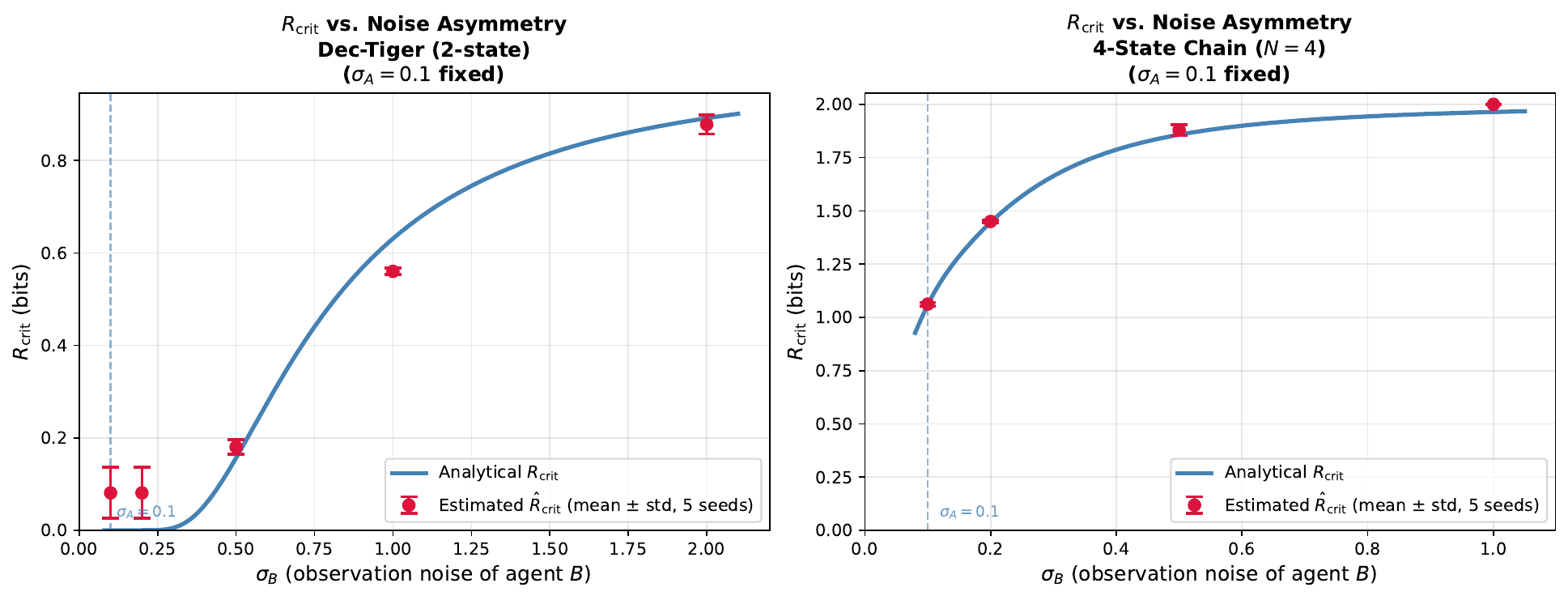
$\hat R_{\rm crit}$ (red, mean$\pm$std over 5 seeds) vs. analytical $H(Q_A\mid Q_B)$ (blue) as $\sigma_B$ increases with $\sigma_A=0.1$. Left: Dec-Tiger. Right: 4-state chain (agent B’s quotient is trivial at $\sigma_B=1.0$, where the estimate is $H(\hat Q_A)=2$ bits).

Limitations

• The guarantee does not cover the procedure that is mostly run. Theorem 1 is about variant (T); the experiments of Sections 5.4–5.7 use procedure (P), for which we have only the partial type-I statement of Section 4.1. Under (T) the analytic threshold is far more conservative and cannot resolve the Gaussian-noise classes at the main sample sizes (Section 5.5).

• The target is resolution-dependent and $B$ must be chosen. In continuous-observation POMDPs the exact history quotient is infinite; the estimator returns the bin-level quotient at the detection scale of the test. Latent indices are recovered when $B$ is aligned with the class structure; with $B$ chosen without $n$ (silhouette or fixed $B=8$) recovery fails on several environments (Section 5.4), and the PO-MuJoCo results certify separability, not a class count.

• One-step keys. All experiments use $\ell=1$; environments in which distinct latent classes share the same observation marginal require $\ell>1$ and $B^\ell$ keys, and we have not evaluated that regime.

• Permutation floor and multiplicity. With $R$ permutations no $p$-value is below $1/(R{+}1)$; family-wise control needs $R\gtrsim K_{\mathrm{hist}}^2/\alpha$, and BH with all $p$-values at the floor rejects everything. The Dec-Tiger over-splits are a direct consequence.

• Single-linkage merging. A single missed split merges two whole classes; a chain of adjacent bins with small pairwise gaps can be merged transitively (observed at $K=16$, $B=32$: $\hat n=12.0\pm3.1<16$).

• $R_{\rm crit}$ proxy. $H(\hat Q_A\mid\hat Q_B)$ is inflated by over-splitting agent A and is a proxy for the rate of Nixon (2026a) only under conditional independence of the observations given the state.

• Alphabet-free, not dimension-free. See Remark 2.

• Observation noise caps partition accuracy. Bins are noisy readouts of the latent state, so the adjusted Rand index of any partition of the bins is bounded (the “ceiling” column of Table 3); ARI measures the combination of bin quality and merging.

• Baselines are re-implementations. The RKHS $\varepsilon$-machine, causal-state and DBC baselines follow the cited estimators but are our code, in the one-observation-past setting; the reward proxy for DBC and the Ferns metric on reward-free environments is a choice of ours (Section 5.6).

Conclusion

We studied Myhill–Nerode quotient learning for continuous observation–action spaces with a kernel-MMD two-sample test on quantile-binned histories. The idea of clustering predictive distributions with MMD is not new (Brodu and Crutchfield 2022); our contribution is a finite-sample formulation with an explicit target (the bin-level quotient at the test’s resolution), an alphabet-free bound for an analysed variant, and an empirical characterisation of when the implemented procedure does and does not recover the latent partition. Directions: bin-count selection with statistical guarantees (silhouette and fixed $B$ both fail on some environments), a guarantee for the permutation/BH procedure, longer history keys ($\ell>1$), and a multi-agent $R_{\rm crit}$ estimator robust to over-splitting.

Proofs of Lemma 1 and Theorem 1

Throughout, $\kappa^2=\sup_x\kappa(x,x)$ and, as required by Gretton et al. (2012, Thm. 7), $0\le\kappa(x,y)\le\kappa^2$; the RBF kernel satisfies both with $\kappa=1$. For a distribution $P$ let $\mu_P=\mathbb{E}_P[\phi(c)]$ be its mean embedding, so that $\mathrm{MMD}(P,Q)=\|\mu_P-\mu_Q\|_{\mathcal{H}_k}$.

Lemma 1: MMD is dominated by total variation

Proof. For $\|f\|_{\mathcal{H}_k}\le1$, $|f(x)|=|\langle f,\phi(x)\rangle|\le\kappa$, hence

$$\mathrm{MMD}(P,Q)=\sup_{\|f\|\le1}\Big|\int f\,d(P-Q)\Big| \le\kappa\,\|P-Q\|_1=2\kappa\,\mathrm{TV}(P,Q).$$

For the second claim, $P_b=\int P^{(k)}_{h',\pi}\,\nu_b(dh')$ where $\nu_b$ is the conditional law of the history given the bin, so $\mu_{P_b}=\int\mu_{P_{h'}}\nu_b(dh')$ (Bochner integral; the embedding is bounded) and

$$\|\mu_{P_h}-\mu_{P_b}\|_{\mathcal{H}_k}\le\int\|\mu_{P_h}-\mu_{P_{h'}}\|\,\nu_b(dh') \le2\kappa\int\mathrm{TV}(P_h,P_{h'})\,\nu_b(dh')\le2\kappa L\,w_b .\qedhere$$

 ◻

Two facts about the biased MMD statistic

Let $X=(x_1,\dots,x_m)\sim P^{\otimes m}$ and $Y=(y_1,\dots,y_m)\sim Q^{\otimes m}$ be independent and let $\widehat{\mathrm{MMD}}$ be the square root of the biased statistic (Eq. (1) of the main paper, $m_1=m_2=m$).

For every $t>0$, $\Pr\big[\,|\widehat{\mathrm{MMD}}-\mathrm{MMD}(P,Q)|>4\kappa/\sqrt m+t\,\big]\le2\exp(-t^2m/(4\kappa^2))$.

If $P=Q$ then, for every $\alpha_0\in(0,1)$, $\Pr\big[\widehat{\mathrm{MMD}}>t_{\alpha_0}\big]\le\alpha_0$ with $t_{\alpha_0}=\sqrt{2\kappa^2/m}\,\big(1+\sqrt{2\log(1/\alpha_0)}\big)$.

Per-pair power

Lemma 2 (Per-pair decision). *Fix $\alpha_0,\delta'\in(0,1)$ and decide “different” iff $\widehat{\mathrm{MMD}}>t_{\alpha_0}$. (i) If $P=Q$ the decision is wrong with probability at most $\alpha_0$. (ii) If $\mathrm{MMD}(P,Q)\ge\varepsilon>0$ and

$$m\;\ge\;\frac{16\kappa^2}{\varepsilon^2}\Big(8+\log\frac{2}{\alpha_0\delta'}\Big),$$

the decision is wrong with probability at most $\delta'$.*

Proof. (i) is Fact in Appendix A.2. For (ii) put $t=2\kappa\sqrt{\log(2/\delta')/m}$, so that $2\exp(-t^2m/(4\kappa^2))=\delta'$. By Fact in Appendix A.2, with probability at least $1-\delta'$, $\widehat{\mathrm{MMD}}\ge\varepsilon-4\kappa/\sqrt m-t$, and the decision is correct as soon as $\varepsilon-4\kappa/\sqrt m-t>t_{\alpha_0}$, i.e.

$$\sqrt m\,\varepsilon\;>\;\kappa\Big[4+\sqrt2+2\sqrt{\log(1/\alpha_0)}+2\sqrt{\log(2/\delta')}\Big].$$

Using $(a+b+c+d)^2\le4(a^2+b^2+c^2+d^2)$ the right-hand side squared is at most $\kappa^2\big[4(4+\sqrt2)^2+16\log(1/\alpha_0)+16\log(2/\delta')\big] \le\kappa^2\big[128+16\log(2/(\alpha_0\delta'))\big]$, and Eq. (3) guarantees $m\varepsilon^2$ exceeds this bound. ◻

Proof of Theorem 1

Proof. Let $\mathcal{P}$ be the set of tested pairs, $|\mathcal{P}|\le K_{\mathrm{hist}}^2/2$. Run the decision of Lemma 2 on every pair with $\alpha_0=\delta'=\delta/K_{\mathrm{hist}}^2$. With $\varepsilon=\varepsilon_{\mathrm{MMD}}$, Eq. (3) becomes $m\ge m_\star$, where $m_\star=(16\kappa^2/\varepsilon_{\mathrm{MMD}}^2)(8+\log(2K_{\mathrm{hist}}^4/\delta^2))$, provided every active bin supplies at least $m_\star$ i.i.d. samples per side from $P_b$; the next paragraph shows when the per_traj sampler does. By a union bound the probability that some pair is decided wrongly is at most $|\mathcal{P}|(\alpha_0+\delta')\le(K_{\mathrm{hist}}^2/2)(2\delta/K_{\mathrm{hist}}^2)=\delta$. On the complementary event every same-class pair (in $\mathcal{Q}^*_B$) is merged and no cross-class pair is merged, so the connected components of the union–find graph are exactly the classes of $\mathcal{Q}^*_B$, i.e. $\widehat{\mathcal{Q}}_B=\mathcal{Q}^*_B$.

Trajectory budget (variant (T), per_traj). Condition on the design half, which fixes the edges, the bandwidth, the active bins $\mathcal{B}$, their pooled laws $P_b$ and masses $\pi_b$ (the pooled mass of $\{z\in b\}$ over $(\text{trajectory},\text{time})$; for equal-length trajectories this is the probability that a uniformly chosen time falls in $b$). The test half contains $N_{\rm t}=N-\lfloor N/2\rfloor\ge N/2$ trajectories; for a pair, a fresh uniformly random half of size $N_s=\lfloor N_{\rm t}/2\rfloor\ge N/4-1\ge N/5$ ($N\ge20$) supplies each side. Each trajectory independently draws one uniform time $t^\star$ and contributes the window starting at $t^\star$ to the bin of $z(o_{t^\star})$. Hence the number of side-$j$ samples in bin $b$ is $\mathrm{Bin}(N_s,\pi_b)$, and, given the counts, those samples are i.i.d. draws from $P_b$ (the conditional law of the window given that the chosen time lies in $b$, which is the pooled bin law of Definition 4), and are independent across sides (disjoint trajectories) and of the design half. No mixing assumption is used. The chain of reasoning in the first paragraph applies with $m=\min(\text{counts})$ on the event $\mathcal E=\{\text{all counts}\ge m_\star\}$, where $m_\star$ is the right-hand side of Eq. (3) with $\varepsilon=\varepsilon_{\mathrm{MMD}}$ (the code subsamples both sides to the common size $m$ uniformly without replacement, which preserves the i.i.d. property). By the multiplicative Chernoff bound $\Pr[\mathrm{Bin}(n,\pi)\le n\pi/2]\le e^{-n\pi/8}$. If $N\ge10m_\star/\pi_{\min}$ then $N_s\pi_b/2\ge N\pi_{\min}/10\ge m_\star$, so each count exceeds $m_\star$ except with probability $\le e^{-N_s\pi_{\min}/8}\le e^{-N\pi_{\min}/40}$. Since $\varepsilon_{\mathrm{MMD}}\le2\kappa$, $m_\star\ge4(8+\log(2K_{\mathrm{hist}}^4/\delta^2))$, so $N\pi_{\min}/40\ge m_\star/4\ge8+\log(2K_{\mathrm{hist}}^4/\delta^2)$ and $e^{-N\pi_{\min}/40}\le e^{-8}\delta^2/(2K_{\mathrm{hist}}^4)$. A union bound over at most $K_{\mathrm{hist}}^2/2$ pairs and 2 sides gives $\Pr[\mathcal E^c]\le K_{\mathrm{hist}}^2 e^{-N\pi_{\min}/40}\le e^{-8}\delta^2/(2K_{\mathrm{hist}}^2)\le\delta$. Together with the pair-decision failure probability $\le\delta$ (which holds conditionally on the counts on $\mathcal E$), $\Pr[\widehat{\mathcal{Q}}_B\ne\mathcal{Q}^*_B]\le2\delta$.

Quantile edges. For $\ell=1$ the design half fits $\hat e_j=F_{N_d}^{-1}(j/B)$ with $N_d=\lfloor N/2\rfloor$. By the DKW argument of Section B (applied to the i.i.d. blocks $G_i$) $\sup_x|F_{N_d}-F|\le t:=\sqrt{\log(2/\delta)/(2N_d)}$ with probability $\ge1-\delta$, and $F$ atomless gives $|F_{N_d}(\hat e_j)-j/B|\le1/(N_dT)$, so $\pi_b\ge1/B-2t-2/(N_dT)$. If $N_d\ge32B^2\log(2/\delta)$, then $t\le1/(8B)$ and $2/(N_dT)\le1/(4B)$, hence $\pi_{\min}\ge1/(2B)$, which holds when $N\ge65B^2\log(2/\delta)$. Substituting $\pi_{\min}\ge1/(2B)$ in Eq. (2) and $K_{\mathrm{hist}}\le B$ gives $N=O(B\log(B/\delta)/\varepsilon_{\mathrm{MMD}}^2+B^2\log(1/\delta))$ with total failure probability $\le3\delta$. The $B^2$ term comes from this crude edge-stability argument and is not claimed to be tight. If the implementation caps each side at $m_{\max}$ samples (the per_traj variant used in the experiments does not), the theorem applies with $m=\min(m,m_{\max})$, i.e. it requires $m_{\max}\ge m_\star$. ◻

Remark 5 (Why the constants matter). With $\kappa=1$, $K_{\mathrm{hist}}=8$, $\delta=0.05$ the per-pair requirement is $m\ge(16/\varepsilon_{\mathrm{MMD}}^2)(8+\log(2\cdot8^4/0.05^2))\approx 400/\varepsilon_{\mathrm{MMD}}^2$. At the sample cap $m_{\max}=300$ used in the experiments this guarantees detection only for $\varepsilon_{\mathrm{MMD}}\gtrsim1.15$; the permutation test is far less conservative than the analytic threshold in practice, but the calculation shows that distinctions with small MMD gaps are not resolved at $m_{\max}=300$, which is the mechanism behind Remark 4 of the main paper. This calculation applies to procedure (P) and to any sampler that caps each side at $m_{\max}$; the per_traj variant of Theorem 1 is uncapped, and its sample budget is the one derived in the proof above.

Proof of Proposition 1 (corrected)

Setting: $\ell=1$; a history is keyed by the bin of the scalar $z=z(o_t)$; the POMDP has finite latent index $n$ with class map $c$; $F$ is the pooled CDF of $z$ (over trajectories and time steps) and $F_N$ its empirical counterpart. Empirical edges are $\hat e_j=F_N^{-1}(j/B)$ and population edges $e_j=F^{-1}(j/B)$, $j=1,\dots,B-1$.

Notation.

$F$ is atomless; population bin $j$ is $(e_{j-1},e_j]$ with $F(e_j)=j/B$ (so each has mass $1/B$). A bin is pure if $z$ falls in a single $I_i$ with probability one on it, and straddling otherwise.

Glivenko–Cantelli.

The $N$ trajectories are i.i.d. blocks of $T$ observations, so $F_N(x)=N^{-1}\sum_i G_i(x)$ with $G_i(x)=T^{-1}\sum_t\mathbf 1\{z^{(i)}_t\le x\}$ i.i.d. in $i$; the class $\{x\mapsto G_i(x)\}$ is monotone and bounded, so $\sup_x|F_N(x)-F(x)|\to0$ almost surely, and (DKW applied to the i.i.d. $G_i$) $\sup_x|F_N(x)-F(x)|=O_P(N^{-1/2})$ for fixed $T$.

Part (i): under (a) only.

Let $G_i=(\sup I_i,\inf I_{i+1})$, $i<n$, be the gaps. A bin intersecting two classes must contain a whole gap in its interior, and a gap lies in the interior of at most one bin, so there are at most $n-1$ straddling bins. Pure bins of the same class share the law $P_i$. Hence the number of distinct bin laws is at most $n$ (pure laws) $+\,(n-1)$ (straddling bins), and trivially at most $B$: $|\mathcal{Q}^*_B|\le\min\{B,2n-1\}$. For the lower bound let $p_i\ge2/B$. Class $i$ occupies the interval of $F$-mass $[q_{i-1},q_i]$ of length $p_i\ge2/B$; the bins are the cells $[(j{-}1)/B,j/B]$ in $F$-mass, and any interval of length at least $2/B$ contains a complete cell, which is then a pure bin of class $i$. So $n$ distinct pure laws exist ($P_i\neq P_{i'}$ by assumption) and $|\mathcal{Q}^*_B|\ge n$. The condition $p_i\ge2/B$ forces $B\ge2n$; if the classes are only known to satisfy $p_i\ge1/B$ (so $B\ge n$), a complete cell is guaranteed only when the class boundaries are cell-aligned, i.e. under (b); without either condition a class of mass $<1/B$ can be spread over two straddling bins and the lower bound $n$ can fail. For $B<n$ the bound $n\le|\mathcal{Q}^*_B|$ is impossible since $|\mathcal{Q}^*_B|\le B$; this is the counterexample to the statement of the earlier version (it assumed $n\le|\mathcal{Q}^*_B|$ with no condition on $B$).

Part (ii): under (a) and (b).

By (b) the level $q_i=F(\sup I_i)=j_i/B$ for an integer $j_i$, and $F$ is constant on $\overline{G_i}$ at level $q_i$, so the population edge $e_{j_i}=F^{-1}(j_i/B)$ lies in $\overline{G_i}$. Hence every population bin is contained in one $I_i$: all bins are pure and $P_b=P_{c(b)}$. The class masses are $p_i=q_i-q_{i-1}$, positive multiples of $1/B$, so $p_i\ge1/B$ (and $n/B\le\sum_ip_i=1$ gives $B\ge n$); every class owns at least one bin and $\mathcal{Q}^*_B$ is the class partition with $|\mathcal{Q}^*_B|=n$.

Part (iii): empirical bins, what is and is not proved.

The empirical edges are $\hat e_j=F_N^{-1}(j/B)$. For the boundary $i$, $F_N(\sup I_i)-q_i=O_P(N^{-1/2})$. The empirical edge $\hat e_{j_i}$ falls in the gap only if $F_N(\sup I_i)$ equals $j_i/B$ exactly; otherwise it falls inside $I_i$ or $I_{i+1}$ and the number of observations of the neighbouring class on the wrong side is $O_P(T\sqrt N)$. Each bin holds $NT/B$ observations, so the foreign-class fraction of every empirical bin is $O_P(B/\sqrt N)$: this tends to zero but is, in general, non-zero at every finite $N$ (equality $F_N(\sup I_i)=j_i/B$ is a lattice event whose probability does not approach one). We therefore do not claim exact purity of empirical bins, and the earlier statement that “with probability $\to1$ every non-empty bin is pure” is not established by this argument and is withdrawn. By the mixture identity $\mathrm{MMD}(\lambda P+(1-\lambda)P',P)=(1-\lambda)\mathrm{MMD}(P,P')$ the MMD between an empirical bin’s law and its class law is $O_P(B/\sqrt N)$.

Run variant (T) with i.i.d. per-bin sample size $m_N=\Theta(N)$ and level $\alpha_N\to0$, $\log(1/\alpha_N)/m_N\to0$. The null threshold is $t_{\alpha_N}=\sqrt{2\kappa^2/m_N}\,(1+\sqrt{2\log(1/\alpha_N)})$, so $\sqrt{m_N}\,t_{\alpha_N}\to\infty$ while the contamination contributes $\sqrt{m_N}\cdot O_P(B/\sqrt N)=O_P(1)$. Same-class pairs have $\widehat{\mathrm{MMD}}\le O_P(m_N^{-1/2})+O_P(B/\sqrt N)<t_{\alpha_N}$ eventually and are merged; cross-class pairs have a gap $\varepsilon-O_P(B/\sqrt N)\to\varepsilon>0$ while $t_{\alpha_N}\to0$, so by Fact in Appendix A.2 they are split with probability $\to1$. A union bound over the finitely many pairs gives $\Pr[\widehat{\mathcal{Q}}_B=\mathcal{Q}^*_B]\to1$ (as a partition of bin indices). This is the precise sense of the recovery claim: vanishing contamination below the detection threshold, not purity.

Under (a) alone, estimation.

If class masses satisfy $p_i\ge2/B$, the lower bound of part (i) holds, the straddling bins’ mixture weights are $N$-independent, and the recovery argument above applies verbatim to $\mathcal{Q}^*_B$ with $|\mathcal{Q}^*_B|\in[n,2n-1]$.

Without (a): unbounded noise.

If the class-conditional laws of $z$ have overlapping supports (e.g. Gaussian noise), $F$ is strictly increasing, every bin contains observations of at least two classes with fixed positive proportions, and the bin laws are proper mixtures whose weights do not depend on $N$. The bound $\Pr[\text{cross}]\le2e^{-\Delta^2/(8\sigma^2)}$ for sub-Gaussian noise with class-mean gap $\Delta$ bounds the proportion of foreign observations in a boundary bin by $\approx2Be^{-\Delta^2/(8\sigma^2)}$; this proportion is constant in $N$, so a consistent test eventually splits the boundary bin (an earlier version of this proposition claimed the proportion vanishes by Borel–Cantelli, which is false). Generically all bin laws are then distinct and $|\mathcal{Q}^*_B|=K_{\mathrm{hist}}$; the finite-sample estimate is a coarsening at the test’s resolution (Remark 4 of the main paper), which is the regime of all Gaussian-noise experiments in the paper.

The environments of the paper.

K-cycle: $z=o=s/K+\xi$, classes of equal mass $1/K$; with $B=K$ the population edges are $F^{-1}(j/K)$, which by the symmetry of the equal-weight mixture lie at the midpoints $(j-\tfrac12)/K$ up to exponentially small tail terms, so (b) holds approximately while (a) fails ($\xi$ Gaussian). Gaussian-mixture random walk: uniform stationary law, $B=N_s$, same situation. Tiger: symmetric marginal, so the median edge is at $0$ and any even $B$ is aligned with the sign boundary. Chain and Dec-Tiger: $B=4$ aligned as above.

Experimental Details

Common defaults (ContinuousEstimatorConfig): history length $\ell=1$, window $k=2$, $m_{\min}=20$, $m_{\max}=300$ continuation vectors per side (deterministic per-pair subsampling), RBF kernel with the median heuristic $2\sigma^2=\mathrm{median}\{\|x-y\|^2\}$ over at most 500 pooled points, permutation $p$-value $(1+\#\{\ge\})/(R+1)$, Benjamini–Hochberg at level $\alpha$ over all pairs. Deviations are listed per experiment.

Tiger (envs/tiger_continuous.py)

States $\{\text{Left},\text{Right}\}$, uniform initial state; actions $\{\text{listen},\text{open-left},\text{open-right}\}$; an open action re-draws the state uniformly. Observation $o=\mathrm{sgn}\cdot1+\mathcal N(0,\sigma^2)$ with $\mathrm{sgn}=-1$ (Left), $+1$ (Right), $\sigma=0.5$. Uniform-random policy, $T=20$. Latent index $n=2$. Estimator: $B=8$ (package default), $\alpha=0.01$, $R=199$. Main run: $N=3000$, 10 seeds (layer1_ground_truth/results/tiger_continuous.csv); $N$-sensitivity: $N\in\{1000,3000,10000\}$, 5 seeds (tiger_N_sensitivity.csv); ablation: $N\in\{500,1000,2000,5000\}$, 3 seeds, $B=2$, $\alpha=0.05$, $R=99$ (baselines/results/ablation_sample_efficiency.csv).

K-cycle (envs/kcycle_continuous.py)

States $\{0,\dots,K-1\}$, deterministic increment mod $K$, uniform initial state; observation $o=s/K+\mathcal N(0,0.1^2)$ (equally spaced means; the $\sin(2\pi s/K)$ variant used in an earlier draft is not injective for even $K$ and is not used); single null action; $T=50$. Latent index $n=K$. Estimator: $B=K$, $\alpha=0.01$, $R=199$, $N=3000$ ($5000$ for $K=16$), 10 seeds (kcycle_continuous.csv). Bin sensitivity: $B=2K$, 5 seeds (kcycle_bins_sensitivity.csv).

Gaussian-mixture random walk (envs/gaussian_mixture_pomdp.py)

$N_s\in\{3,4,5,6\}$ states, $s'=\mathrm{clip}(s+\delta,0,N_s-1)$, $\delta\sim\mathrm{Unif}\{-1,0,1\}$; $o=s+\mathcal N(0,0.15^2)$; $T=50$, $N=2000$; $\alpha=0.05$, $R=99$; $B=N_s$ (manual) and $B$ auto-selected by silhouette over $\{2,\dots,32\}$ (Algorithm 2 below); 5 seeds (gaussian_mixture.csv).

PO-HalfCheetah and PO-Ant (layer2_mujoco/)

HalfCheetah-v4: 17-dim observation (8 joint positions, 9 joint velocities); the wrapper zeroes indices $0$–$8$, leaving 8 velocity coordinates. Ant-v4: 27-dim observation; indices $13$–$26$ (14 velocities) are kept. Zero-torque policy (and, for HalfCheetah, torques $\propto\sin(\omega t+\phi_i)$ per joint); $N=5000$, $T=50$, $B=8$, $\alpha=0.05$, $R=99$, 5 seeds (halfcheetah_continuous.csv, halfcheetah_sinusoidal.csv, ant_continuous.csv); auto-bin: 3 seeds (halfcheetah_autobin.csv).

Class statistics and value prediction are in halfcheetah_class_returns.csv, halfcheetah_value_prediction.csv and halfcheetah_sinusoidal_value.csv. The binning scalar is $z(o)=\|o\|_2$ (velocity norm). No discretised G-test baseline is reported: no result file exists for it.

Dec-Tiger and chain Dec-POMDPs (layer3_rcrit/)

Both agents run a listen-only policy so the latent state is constant within an episode; $N=1000$, $T=20$, $B=4$, $m_{\min}=10$, $\alpha=0.05$, $R=99$. Dec-Tiger: $o^i=\mathrm{sgn}+\mathcal N(0,\sigma_i^2)$; chain: 4-state random walk (uniform stationary law), $o^i=s/4+\mathcal N(0,\sigma_i^2)$. Each agent’s quotient is fitted independently; each step is labelled by the class of its binned key; $\hat R_{\rm crit}=H(\hat Q_A,\hat Q_B)-H(\hat Q_B)$ (plug-in entropies, clamped at $0$).

Analytical $H(Q_A\mid Q_B)$.

Dec-Tiger: $Q_i=\mathrm{sign}(o^i)$ (the $B=4$ quantile edges of a symmetric marginal put the middle edge at $0$), so $p_i=\Pr[Q_i\ne s]=\Phi(-1/\sigma_i)$. With $\Pr[s=\pm1]=\tfrac12$,

$$\begin{aligned} \Pr(Q_A=Q_B=s) &=\tfrac12(1-p_A)(1-p_B)+\tfrac12p_Ap_B \quad(\text{each sign}),\\ \Pr(Q_A\ne Q_B) &=\tfrac12(1-p_A)p_B+\tfrac12p_A(1-p_B)\quad(\text{each pattern}), \end{aligned}$$

and $H(Q_A\mid Q_B)=H(Q_A,Q_B)-H(Q_B)$. Symmetric $\sigma=0.5$: $p=\Phi(-2)=0.0228$, $H(Q_A\mid Q_B)=0.2624$ bits. Asymmetric $(\sigma_A,\sigma_B)=(0.1,1.0)$: $p_A=\Phi(-10)\approx0$, $p_B=\Phi(-1)=0.1587$, $H(Q_A\mid Q_B)=H_b(0.1587)=0.6311$ bits; ratio $2.41$. Sweep values ($\sigma_A=0.1$): $\sigma_B=0.1,0.2,0.5,1.0,2.0\mapsto0.0000,0.0000,0.1566,0.6311,0.8915$. (An earlier draft wrote these formulas with a threshold at $0.5$ and $\Phi(-0.5/\sigma)$; that does not match the environment or the numbers.) Chain: agent $i$ classifies $s$ by the nearest mean, i.e. intervals with edges $(2s+1)/8$; $\Pr(Q_i=j\mid s)=\Phi((\text{hi}_j-s/4)/\sigma_i)-\Phi((\text{lo}_j-s/4)/\sigma_i)$; joint over uniform $s$; values $\sigma_B=0.1,0.2,0.5,1.0\mapsto1.0584,1.4462,1.8576,1.9642$ bits.

Baselines (experiments/revision/baselines_lib.py)

All baselines see the same trajectories as the quotient estimator, are scored by the adjusted Rand index against the latent state, and none uses $n$ (except the “$B=n$” reference rows). They are our re-implementations of the cited estimators in the same one-observation-past setting, not the authors’ code.

• $W_1$ (multivariate). Bin-conditional continuation vectors ($d_c=3$: $o_{t+1},a_{t+1},o_{t+2}$, raw units), at most 300 per bin; exact Wasserstein-1 between equal-size subsamples via optimal assignment under the Euclidean cost. Bins are merged if $W_1<\varepsilon$ with $\varepsilon\in\{0.1,0.2,0.5,1.0\}$ (single linkage, as for the quotient estimator), or parameter-free by average-linkage clustering of the $W_1$ matrix with the number of clusters chosen by silhouette.

• Ferns bisimulation metric. The finite-MDP metric of Ferns et al. (2004) (the continuous-space metric of Ferns et al. (2011) cannot be computed from samples without an abstraction), on the empirical chain over the $B$ quantile bins: $d_{n+1}(s,t)=\max_a[(1-c)|r(s,a)-r(t,a)|+c\,W_1(P(\cdot|s,a),P(\cdot|t,a);d_n)]$, $c=0.9$, exact LP for $W_1$, fixed point by iteration (tolerance $10^{-6}$, at most 40 sweeps), rewards rescaled to $[0,1]$. Bins are clustered by average linkage with silhouette selection of the number of clusters.

• DBC. The objective of Zhang et al. (2021) without the RL learner: MLP encoder ($1\to64\to64\to8$), Gaussian latent dynamics model $\hat P(z'|z,a)$ trained by negative log-likelihood on stop-gradient encoded next observations, and the loss $(\|z_i-z_j\|_1-|r_i-r_j|-\gamma W_2(\hat P(\cdot|\bar z_i,a_i),\hat P(\cdot|\bar z_j,a_j)))^2$ on random pairs within a batch of 256, $\gamma=0.99$, 3000 Adam steps. Classes: $k$-means on the embedding of every step with $k\in[2,12]$ by silhouette.

• Reward for DBC and the Ferns metric. Bisimulation is reward-defined. Tiger uses its native reward; the K-cycle and GaussMix environments are reward-free, so we use the next observation $o_{t+1}$ as an emission reward. Both are rescaled to $[0,1]$ (DBC, Ferns) — this is our choice and affects those baselines.

• Causal-state learning. Following Zhang et al. (2019): a GRU (hidden size 32) reads $(o_{\le t},a_{<t})$, a head predicts $o_{t+1}$ (and the reward on Tiger) from $(h_t,a_t)$ by mean squared error (30 epochs, Adam, batch 128 trajectories); the hidden states are discretised by $k$-means with $k\in[2,12]$ by silhouette (one of the two discretisers described in their Sec. 4.2). It conditions on the full history, unlike the other methods.

• RKHS $\varepsilon$-machine. Following Brodu and Crutchfield (2022), past $=$ present observation, future $=$ the $k=2$ continuation vector, 1500 randomly drawn $(x,y)$ pairs, Gaussian kernels $\exp(-\|\cdot\|^2/\xi^2)$ with $\xi=$ median pairwise distance; weights $\Omega=(G^X+\varepsilon I)^{-1}G^X$ with $\varepsilon\in\{10^{-4},\dots,1\}$ by 3-fold cross-validation of the held-out embedding error; $G^S=\Omega^\top G^Y\Omega$; diffusion-map coordinates (density-normalised, row-stochastic, spectral-gap truncation); clustering by DBSCAN with $\varepsilon_{\rm DB}=0.1\times$ the range of the leading coordinate (their DBSCAN with threshold $0.1$ is on unnormalised coordinates; our rescaling is a choice) or by $k$-means with silhouette.

• Legacy baselines. The first-coordinate-projection Wasserstein and the custom Wasserstein-matching DBC objective of the previous version (bisim_comparison.csv, dbc_comparison.csv) are superseded and no longer used; the G-test rows come from ablation_sample_efficiency.csv.

Revision experiments (variant (T), partition accuracy)

Data: the same generators and settings as Appendix C (Tiger $N{=}3000$, $T{=}20$, $\alpha{=}0.01$, $R{=}199$; K-cycle $N{=}3000$, $T{=}50$, $\alpha{=}0.01$, $R{=}199$; GaussMix $N{=}2000$, $T{=}50$, $\alpha{=}0.05$, $R{=}99$), random policy, with the latent state recorded for scoring (the action space is seeded here; the original runs sampled actions from an unseeded action-space generator, so individual draws differ from the earlier result files). Seeds $0$–$4$. Procedure (P): the package estimator unchanged. Variant (T) and (P$^{\rm fix}$): continuous_quotient/variant_t.py, $\delta=0.05$ for (T), $\alpha$ and $R$ as for (P) for (P$^{\rm fix}$), design fraction $0.5$, minimum $20$ samples per side. Sampler: the (T-pt) and P$^{\rm fix}$-pt rows use per_traj (the sampler Theorem 1 covers); the (T-pb) rows and the old P$^{\rm fix}$ comparison in partition_accuracy.csv use per_bin (not covered); Dec-Tiger uses per_traj. ARI is computed over all steps with a full 2-step continuation whose bin is active. Result files: partition_accuracy.csv (merged from partition_accuracy_part1.csv, _part2.csv, _part3.csv by summarize.py), partition_baselines.csv, tiger_T_scaling.csv, dec_tiger_variant_t.csv, and, added with the per_traj analysis of this version, partition_accuracy_pertraj.csv, partition_accuracy_2n.csv, T_traj_scaling.csv, tiger_T_scaling_pertraj.csv and dec_tiger_pfix_N20000_seeds3_9.csv.

Additional Results

Auto bin selection

Trajectories, $B_{\min}=2$, $B_{\max}=32$, subsample size 2000. $k$-means with $B$ clusters on the subsampled binning scalars $z(o)$; silhouette score $s_B$. $\arg\max_Bs_B$.

Silhouette measures cluster quality in observation space and is a heuristic proxy for the number of latent classes; it under-estimates $B$ when classes share observation marginals. Results (this revision, partition_accuracy.csv): silhouette selects $B=2$ on Tiger, $B=K$ for K-cycle $K\in\{2,3\}$ but $B=2$ for $K\in\{4,5,8\}$ (5 seeds each), and $B=N_s$ on GaussMix. (The previous version’s claim of $B=K$ on K-cycle had no result file.) Earlier GaussMix results—$B=N_s$ on all 20 runs, and the auto-$B$ estimate equals the manual one on every run (gaussian_mixture.csv); PO-HalfCheetah (passive)—$B=3$ on all 3 seeds with $\hat n=3,3,2$ (halfcheetah_autobin.csv).

K-cycle per-seed results and runtime

K-cycle at $B=K$ (kcycle_continuous.csv): all 60 runs return $\hat n=K$. Wall-clock per run on one CPU core.

K-cycle at $B=2K$, 5 seeds (kcycle_bins_sensitivity.csv). Over-provisioned bins are split whenever the half-class bins’ posteriors differ detectably ($3\le K\le8$); at $K=16$ the 32 bins are close enough that single-linkage chaining merges neighbours and the estimate falls below $K$.

Tiger vs. $N$

$B=8$, $\alpha=0.01$, $R=199$, 5 seeds (tiger_N_sensitivity.csv): $\hat n=2$ on every seed at $N=1000$, $3000$ and $10000$. Ablation runs ($B=2$, $\alpha=0.05$, $R=99$): $\hat n=2$ on 3/3 seeds at every $N\in\{500,1000,2000,5000\}$.

Dec-Tiger per-seed results

Dec-Tiger, $\alpha=0.05$, $R=99$, all seeds (dec_tiger_asymmetric.csv; seeds 0–4 of the symmetric block are also in dec_tiger_rcrit.csv). Analytical: $0.2624$ (symmetric), $0.6311$ (asymmetric).

Over-splitting of agent A ($\hat n_A=3$) triples the estimate; over-splitting of agent B is harmless. The mechanism is the resolution effect: with $\sigma=0.5$ the posteriors of the two same-side bins differ by up to $\approx0.05$ in posterior weight (the $B{=}4$ quantile bins of a $\pm1$, $\sigma{=}0.5$ marginal give $\Pr(\text{Right}\mid b)\approx0.0001$ and $0.045$ for the two left-side bins), at the edge of what $R=99$ permutations and $m_{\max}=300$ resolve, and BH with only six $p$-values rejects all of them once all six reach the floor $1/(R+1)=0.01$. Table 14 reports the sensitivity run at $\alpha=0.01$ with $R=999$ (at $R=99$ the floor equals $\alpha$ and every quotient collapses to one class).

Dec-Tiger, $\alpha=0.01$, $R=999$, 10 seeds (dec_tiger_sym_alpha001_R999.csv, dec_tiger_asym_alpha001_R999.csv).

Noise sweep per level

Sweep, $\sigma_A=0.1$, 5 seeds per level (rcrit_sweep.csv, chain_rcrit.csv). Relative errors are undefined when the analytical value is $0$; absolute errors are given.

Neural encoder

The code ships a GRU/InfoNCE history encoder (neural_encoder.py) trained on the MMD partition; no results for it are reported in this paper because no result files were produced.

PO-HalfCheetah class statistics and value prediction

Tables 16–18 follow. Their $R^2$ values are in-sample fits on all time steps; the held-out, trajectory-level analysis against a nonlinear speed baseline is in Table 9 of the main paper (halfcheetah_groupsplit_value.csv, halfcheetah_groupsplit_value.py) and supersedes the interpretation “classes carry multi-step information beyond speed”, which these in-sample linear comparisons do not support.

Per-class statistics for the $n{=}8$ quotient partition on PO-HalfCheetah. Classes are sorted by mean velocity $\ell_2$ norm. $\bar{G}$ = mean discounted return ($\gamma{=}0.99$) from each timestep assigned to that class. Kruskal-Wallis $H=4897.3$, $p \approx 10^{-1055}$ (computed over time steps, which are dependent within trajectories; the $p$-value is not evidence of a trajectory-level effect).

Class-conditioned value prediction on PO-HalfCheetah (zero-action policy, $\gamma=0.99$, $n=51,000$ timesteps). The auto-selected $B=3$ quotient partition explains $1.0\%$ of return variance (linear $R^2$) and $\eta^2=0.010$ of total variance (ANOVA effect size). The Kruskal-Wallis $p$-value ($4.92\times10^{-117}$) treats time steps as independent and is not evidence of a trajectory-level effect. All $R^2$ values here are in-sample; see Table 9 for the held-out, trajectory-level comparison against a nonlinear speed baseline, which shows the classes carry no information beyond speed.

Class-conditioned value prediction on PO-HalfCheetah under the sinusoidal locomotion policy ($\gamma=0.99$, $101{,}000$ time steps; halfcheetah_sinusoidal_value.csv).

Artifacts, result files and corrections

Code, scripts and result files are in the public repository https://github.com/npow/quotient-learning-papers, directory cql/; the artifacts cited here are at tag v1, which points to commit 83f9f42d8533c62fd05fcef2192559e0f80be3d9 (tags can be retargeted; the hash is the immutable reference). Result files and scripts added in this revision (marked “this version” below: partition_accuracy_pertraj.csv, partition_accuracy_2n.csv, T_traj_scaling.csv, tiger_T_scaling_pertraj.csv, dec_tiger_pfix_N20000_seeds3_9.csv and their scripts) are not in v1; they are in commit 2c168297b5cd6fcc35e9a0a6a901411d2d1fb404 of the same repository. All paths below are relative to cql/.

Result files (every number in the paper comes from one of these).

• Layer 1 (experiments/layer1_ground_truth/results/): tiger_continuous.csv, kcycle_continuous.csv, gaussian_mixture.csv, kcycle_bins_sensitivity.csv, tiger_N_sensitivity.csv.

• Layer 2 (experiments/layer2_mujoco/results/): halfcheetah_continuous.csv, halfcheetah_sinusoidal.csv, ant_continuous.csv, halfcheetah_autobin.csv, halfcheetah_class_returns.csv, halfcheetah_value_prediction.csv, halfcheetah_sinusoidal_value.csv (in-sample, superseded), halfcheetah_groupsplit_value.csv (trajectory-level held-out split).

• Layer 3 (experiments/layer3_rcrit/results/): dec_tiger_rcrit.csv, dec_tiger_asymmetric.csv, dec_tiger_sym_alpha001_R999.csv, dec_tiger_asym_alpha001_R999.csv, chain_rcrit.csv, rcrit_sweep.csv.

• Legacy baselines (experiments/baselines/results/): ablation_sample_efficiency.csv (G-test rows only are still used); bisim_comparison.csv and dbc_comparison.csv are the first-coordinate Wasserstein and the custom DBC objective of the previous version and are superseded (not used in any table of this version).

• Table-to-file map: main-paper Table 4 $\leftarrow$ partition_accuracy.csv (P, T-pb) and partition_accuracy_pertraj.csv (T-pt); Tiger scaling in the text $\leftarrow$ tiger_T_scaling_pertraj.csv; K-cycle/GaussMix scaling $\leftarrow$ T_traj_scaling.csv; Dec-Tiger (iv) $\leftarrow$ dec_tiger_variant_t.csv and dec_tiger_pfix_N20000_seeds3_9.csv; Table 1 $\leftarrow$ tiger_continuous.csv, kcycle_continuous.csv, gaussian_mixture.csv; Table 2 $\leftarrow$ kcycle_bins_sensitivity.csv, tiger_N_sensitivity.csv; Table 3 $\leftarrow$ partition_accuracy.csv; Table 6 $\leftarrow$ partition_baselines.csv (with partition_accuracy.csv for the (P) rows); Table 7 $\leftarrow$ ablation_sample_efficiency.csv; Table 8 $\leftarrow$ the Layer 2 files halfcheetah_continuous.csv, halfcheetah_sinusoidal.csv, ant_continuous.csv, halfcheetah_autobin.csv; Table 9 $\leftarrow$ halfcheetah_groupsplit_value.csv; the $R_{\rm crit}$ tables and figure $\leftarrow$ the Layer 3 files (dec_tiger_rcrit.csv, dec_tiger_asymmetric.csv, dec_tiger_sym_alpha001_R999.csv, dec_tiger_asym_alpha001_R999.csv, chain_rcrit.csv, rcrit_sweep.csv).

• Revision (experiments/revision/results/): partition_accuracy.csv (procedures P, and T and P$^{\rm fix}$ with per_bin; ARI), partition_accuracy_pertraj.csv (T and P$^{\rm fix}$ with per_traj), partition_accuracy_2n.csv ($B=2n$ on K-cycle $K\in\{4,5,8\}$: P, P$^{\rm fix}$-pt, T-pt), T_traj_scaling.csv (T-pt as $N$ grows), tiger_T_scaling.csv (per_bin) and tiger_T_scaling_pertraj.csv, dec_tiger_pfix_N20000_seeds3_9.csv (7 additional P$^{\rm fix}$ seeds), partition_baselines.csv (W1, Ferns metric, DBC, causal-state, RKHS $\varepsilon$-machine; ARI), dec_tiger_variant_t.csv, gaussmix_alpha_check.csv.

Scripts: experiments/revision/run_partition_accuracy.py, run_partition_baselines.py, baselines_lib.py, run_dec_tiger_variant_t.py, run_dec_tiger_pfix_extra.py, run_T_traj_scaling.py, run_tiger_T_scaling.py, check_gaussmix_alpha.py, experiments/layer2_mujoco/halfcheetah_groupsplit_value.py; package code continuous_quotient/variant_t.py; tests under tests/.

Corrections to the previous version.

• Table 2, Tiger at $N=10000$. The entry “$2,2,2,2,20$” was a typo. tiger_N_sensitivity.csv contains $\hat n=2$ on all five seeds at $N=10000$ (and $B=8$ makes $\hat n=20$ impossible); the table now reads $2,2,2,2,2$, in agreement with Appendix D.

• GaussMix $\alpha$. The shipped CSV has no $\alpha$ column. The script default is $\alpha=0.05$, Appendix C said $0.05$ and Section 5 said $0.01$. We re-ran the manual-$B$ configuration ($B=N_s$, $R=99$, $N=2000$, seeds 0–2, gaussmix_alpha_check.csv) at both levels: $\hat n=N_s$ on all 12 runs at $\alpha=0.05$ and at $\alpha=0.01$, so the result file cannot discriminate between the two settings and the reported numbers are unaffected. The paper now states $\alpha=0.05$, $R=99$ throughout.

• Missing result-file names in Appendices C–D are filled in above; in the rendered web version of the previous submission every was dropped by our converter, which left the file lists blank.

• Variant (T) sampler (this version). The previous (T) experiments used the per_bin sampler, which does not sample the pooled bin law $P_b$ of Definition 4, so they did not test Theorem 1. Theorem 1 and its trajectory budget were restated for per_traj (Section A) and Table 4 now reports it alongside the old sampler. The per_traj runs are much more conservative at $N\le3000$.

• Pow 2026 / companion paper is unpublished; nothing in this paper’s claims relies on it beyond the definition of the finite-alphabet baseline, and its G-test rows in Table 7 come from ablation_sample_efficiency.csv.

References

1. Abel, David, Nate Umbanhowar, Khimya Khetarpal, Dilip Arumugam, Doina Precup, and Michael Littman. 2020. “State Abstraction as Compression in Apprenticeship Learning.” Proceedings of the 34th AAAI Conference on Artificial Intelligence, 3134–42.
2. Azizzadenesheli, Kamyar, Alessandro Lazaric, and Animashree Anandkumar. 2016. “Reinforcement Learning of POMDP’s Using Spectral Methods.” Proceedings of the 29th Annual Conference on Learning Theory (COLT), 193–256.
3. Benjamini, Yoav, and Yosef Hochberg. 1995. “Controlling the False Discovery Rate: A Practical and Powerful Approach to Multiple Testing.” Journal of the Royal Statistical Society: Series B 57 (1): 289–300.
4. Boots, Byron, Geoffrey Gordon, and Arthur Gretton. 2013. “Hilbert Space Embeddings of Predictive State Representations.” Proceedings of the 29th Conference on Uncertainty in Artificial Intelligence (UAI).
5. Boots, Byron, Sajid M. Siddiqi, and Geoffrey J. Gordon. 2011. “Closing the Learning-Planning Loop with Predictive State Representations.” International Journal of Robotics Research 30 (7): 954–66.
6. Brodu, Nicolas, and James P. Crutchfield. 2022. “Discovering Causal Structure with Reproducing-Kernel Hilbert Space $\varepsilon$-Machines.” Chaos: An Interdisciplinary Journal of Nonlinear Science 32 (2): 023103. https://doi.org/10.1063/5.0062829.
7. Castro, Pablo Samuel. 2020. “Scalable Methods for Computing State Similarity in Deterministic Markov Decision Processes.” Proceedings of the 34th AAAI Conference on Artificial Intelligence, 10069–76.
8. Castro, Pablo Samuel, Prakash Panangaden, and Doina Precup. 2009. “Equivalence Relations in Fully and Partially Observable Markov Decision Processes.” Proceedings of the 21st International Joint Conference on Artificial Intelligence (IJCAI), 1653–58.
9. Ferns, Norm, Prakash Panangaden, and Doina Precup. 2004. “Metrics for Finite Markov Decision Processes.” Proceedings of the 20th Conference on Uncertainty in Artificial Intelligence (UAI), 162–69.
10. Ferns, Norm, Prakash Panangaden, and Doina Precup. 2011. “Bisimulation Metrics for Continuous Markov Decision Processes.” SIAM Journal on Computing 40 (6): 1662–714. https://doi.org/10.1137/10080484X.
11. Goerg, Georg M., and Cosma Rohilla Shalizi. 2012. “LICORS: Light Cone Reconstruction of States for Non-Parametric Forecasting of Spatio-Temporal Systems.” Unpublished manuscript.
12. Goerg, Georg M., and Cosma Rohilla Shalizi. 2013. “Mixed LICORS: A Nonparametric Algorithm for Predictive State Reconstruction.” Proceedings of the 16th International Conference on Artificial Intelligence and Statistics (AISTATS), JMLR workshop and conference proceedings, vol. 31: 289–97.
13. Gretton, Arthur, Karsten M. Borgwardt, Malte J. Rasch, Bernhard Schölkopf, and Alexander Smola. 2012. “A Kernel Two-Sample Test.” Journal of Machine Learning Research 13 (25): 723–73. http://jmlr.org/papers/v13/gretton12a.html.
14. Jaeger, Herbert. 2000. “Observable Operator Models for Discrete Stochastic Time Series.” Neural Computation 12 (6): 1371–98.
15. Jurgens, Alexandra M., and Nicolas Brodu. 2024. “Inferring Kernel $\varepsilon$-Machines: Discovering Structure in Complex Systems.” Unpublished manuscript.
16. Kaelbling, Leslie Pack, Michael L. Littman, and Anthony R. Cassandra. 1998. “Planning and Acting in Partially Observable Stochastic Domains.” Artificial Intelligence 101 (1–2): 99–134.
17. Larsen, Kim G., and Arne Skou. 1991. “Bisimulation Through Probabilistic Testing.” Information and Computation 94 (1): 1–28.
18. Nixon, Anthony T. 2026a. “Semantic Rate-Distortion for Bounded Multi-Agent Communication: Capacity-Derived Semantic Spaces and the Communication Cost of Alignment.” arXiv Preprint arXiv:2604.09521.
19. Nixon, Anthony T. 2026b. “The Myhill–Nerode Theorem for Bounded Interaction: Canonical Abstractions via Agent-Bounded Indistinguishability.” arXiv Preprint arXiv:2603.21399.
20. Pow, Nissan. 2026. “Online Learning of Myhill–Nerode Quotients in Bounded-Agent POMDPs.” Unpublished manuscript.
21. Ramdas, Aaditya, Sashank J. Reddi, Barnabás Póczos, Aarti Singh, and Larry Wasserman. 2015. “On the Decreasing Power of Kernel and Distance Based Nonparametric Hypothesis Tests in High Dimensions.” Proceedings of the 29th AAAI Conference on Artificial Intelligence, 3571–77.
22. Zaremba, Wojciech, Arthur Gretton, and Matthew Blaschko. 2013. “B-Test: A Non-Parametric, Low Variance Kernel Two-Sample Test.” Advances in Neural Information Processing Systems (NeurIPS) 26.
23. Zhang, Amy, Zachary C. Lipton, Luis Pineda, et al. 2019. “Learning Causal State Representations of Partially Observable Environments.” Unpublished manuscript.
24. Zhang, Amy, Rowan McAllister, Roberto Calandra, Yarin Gal, and Sergey Levine. 2021. “Learning Invariant Representations for Reinforcement Learning Without Reconstruction.” International Conference on Learning Representations (ICLR).

Disclosure of AI use

Claude (Anthropic; Claude Code with Sonnet and Opus-class models) was used throughout this work: writing and debugging the code in the linked repository, running and checking experiments, drafting and revising the manuscript, and simulated peer review. The human author directed the research, reviewed the results, and is responsible for the content. All reported numbers are produced by committed scripts.